
If one region fails, a global load balancer can keep your service online by sending users to another healthy region under the same hostname.
I’d sum it up like this: IBM Cloud Global Load Balancers are DNS-based traffic directors. They sit above your regional load balancers, check which regions are healthy, and then send users to the best regional endpoint based on health, location, or latency. For UK teams, that usually means three things: less outage risk, better response times, and one public address for a multi-region service.
Here’s the short version:
- A GLB works at the DNS layer, not inside one region
- It routes users to regional origin pools, such as London or Frankfurt
- Health checks drive failover when a pool stops responding
- Steering modes usually include failover, geo, and dynamic latency
- TTL affects failover timing: 30 seconds can shift traffic far sooner than 300 seconds
- Session affinity can keep users on one pool with cookies
- CIS and DNS Services both support GLB, but CIS also adds security features
- Active-active suits high-traffic customer services; active-passive suits lower-cost disaster recovery
- Quotas matter: for example, the article notes limits such as 5 GLBs per CIS Standard instance and 25 per DNS Services zone
What I take from the article is simple: pick the routing policy, TTL, failover model, and quota plan before rollout. If those four parts are wrong, the setup can look fine on paper but still fail under pressure.
Quick comparison
| Area | What to know |
|---|---|
| Main job | Send users to the best healthy region |
| Best for | Multi-region apps, DR setups, UK/EU traffic routing |
| Routing inputs | Pool health, user location, latency policy |
| Steering options | Failover, geo, dynamic latency |
| User impact | Lower delay, fewer full-service outages, one hostname |
| Main trade-off | Lower TTL gives faster failover but more DNS queries |
| Common setup | GLB → regional pool → regional ALB/NLB/ingress |
| Planning checks | DNS control, health-check paths, source ranges, quotas |
In short, I see IBM Cloud GLB as the layer that decides which region should answer before the regional load balancer decides which backend should answer inside that region.
How IBM Cloud global load balancers route traffic across regions
Those gains come down to one thing: how the GLB picks a regional endpoint for each DNS lookup. An IBM Cloud global load balancer makes DNS decisions across regions. When a user’s device looks up app.example.co.uk, the GLB returns the healthiest regional endpoint for that query - whether that’s London, Frankfurt or Dallas. Three things shape each DNS answer: origin pool health, the user’s location, and the steering mode set by the engineering team.
Origin pools, health checks and failover behaviour
An origin pool groups the endpoints for one region, such as two London VPC load balancers. [1][11]
IBM Cloud health checks mark a pool unhealthy when it fails again and again, then remove it from DNS responses automatically. [3][10][4]
Failover speed depends on the health-check interval and failure threshold. Shorter settings spot outages sooner, but they can also cause fast back-and-forth health changes. Longer settings make routing steadier, but recovery takes more time. [1][11]
Steering modes: failover, geo and dynamic latency
IBM Cloud then applies one of three steering modes to make that choice.
| Steering Mode | Ideal Use Case | Trade-offs | UK Example |
|---|---|---|---|
| Failover | Active-passive disaster recovery | Standby region sits idle; distant users may see higher latency | London payroll system failing over to Frankfurt during an incident |
| Geo | Regulatory compliance, localised content | Harder to map every geography; nearest region may not be the fastest | Banking app keeping UK customers within EMEA data centres |
| Dynamic latency | Performance-critical consumer apps | Traffic can move between regions in ways that are harder to track | E-commerce platform routing London and Manchester users to whichever region responds fastest |
These modes can also work with pool priority. A team, for instance, might use geo routing within EMEA, then fail over to another region if every EMEA pool becomes unhealthy. When dynamic latency steering is first switched on, IBM recommends allowing roughly 10 minutes for latency profiles to build before expecting accurate routing decisions. [12]
TTL and session affinity: practical effects on live traffic
DNS TTL controls how long resolvers cache a GLB response before querying again. A TTL of 30 seconds means a user who cached a London pool IP at 10:00:00 will refresh by roughly 10:00:30 if that pool fails. A TTL of 300 seconds stretches that window to five minutes. [15][5]
Shorter TTLs help failover happen sooner and keep geo or latency steering on track, but they also increase DNS query volume. Longer TTLs cut that load and make routing steadier, but they slow recovery. [15][5]
Session affinity keeps a user tied to the same origin pool for a set period. That matters for stateful apps that need users to stay on one region during a session. In IBM Cloud, this is done through cookie-based affinity: a cookie issued on first contact keeps the user on their assigned pool. If that pool becomes unhealthy, a new cookie is issued pointing to a healthy failover pool, so availability remains protected if the pool fails. [13][14] For stateless microservices, turning session affinity off allows traffic to spread more evenly across regions without any continuity risk.
These routing controls set up the rollout choices and limits covered next.
When teams use IBM Cloud global load balancers for multi-region applications
These routing rules start to make sense once you place them inside real multi-region setups. In IBM Cloud, global load balancers usually show up in two common patterns: multi-region VPC designs and Kubernetes or OpenShift clusters spread across regions. Both use the same routing model, just applied to different kinds of deployments.
Multi-region VPC and load balancer designs
In this setup, each region runs its own VPC, with a regional ALB or NLB sitting in front of the app tier. The global load balancer is then exposed through CIS or DNS Services under one hostname, such as app.company.co.uk, for users across the UK and other locations.[7][17][18]
Each regional ALB or NLB is added as an origin in a pool. A simple example would be separate London and Frankfurt pools, with health checks hitting a path such as /healthz on each endpoint. If London is healthy, UK traffic goes there. If London starts failing health checks, traffic shifts to Frankfurt on its own.[16][17][7]
For workloads with strict data residency rules, geo steering helps keep UK users on UK-based or nearby EMEA infrastructure, while still allowing failover to another region if the preferred one goes unhealthy.[2][9][7]
The same setup works for container platforms too.
Kubernetes and OpenShift across more than one region
Kubernetes and OpenShift deployments follow much the same pattern. Each regional cluster exposes an ingress endpoint, often through NGINX, HAProxy or OpenShift's built-in router, with a regional ALB in front of it. That endpoint is then added as an origin in the global load balancer pool for its region.[6][21][22]
IBM's multi-region Kubernetes guidance describes pools built around UK and US clusters, using geo steering to direct users to the nearest cluster, plus a fallback pool if one cluster becomes unavailable.[6] In an active-active container setup, both clusters serve live traffic at the same time, which helps with resilience and response times. In an active-passive design, the secondary cluster stays ready but idle, and only takes traffic when the primary cluster fails its health checks.
A useful rule here is to expose only external APIs and web front ends, while keeping internal services local to each region.[6][22]
Comparing active-active and active-passive: a short decision guide
Once the topology is set, the next choice is simple: how much traffic should each region handle? Active-active suits teams that want higher availability. Active-passive fits teams that want lower cost and less operational overhead.
| Aspect | Active-active | Active-passive |
|---|---|---|
| Traffic on regional failure | Capacity drops, but there is no total outage; remaining regions take the load | Traffic fails over to the secondary region; a short interruption can happen |
| Deployment complexity | Higher - needs multi-region data replication and consistent configuration | Lower - the primary region is tuned for production, while the secondary focuses on readiness |
| Runbook and monitoring burden | Higher - cross-region deployments, monitoring and fault-finding take more work | More contained - the main task is testing disaster recovery runbooks on a regular basis |
| Recovery behaviour | Fast and mostly automatic - traffic rebalances across the active regions still running | Depends on health-check-triggered or manual failover; users may notice a short interruption |
| Cost profile | Higher baseline - capacity and data services run across all active regions | Lower baseline - the standby region can run with less capacity and scale up only when needed |
For revenue-critical or customer-facing services, active-active is usually the better fit, because a regional failure cuts capacity instead of taking the whole service down. For back-office or lower-traffic systems, where a short recovery window is acceptable, active-passive can keep cost and complexity in check, as long as the team tests failover often and keeps disaster recovery runbooks up to date.[7][19][23]
Configuration steps, limits and planning before rollout
::: @figure 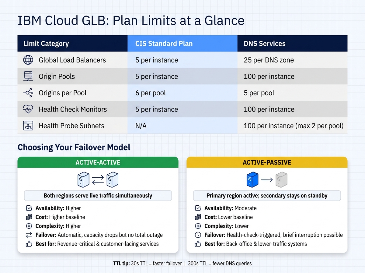 {IBM Cloud GLB: Active-Active vs Active-Passive & CIS vs DNS Services Limits}
:::
{IBM Cloud GLB: Active-Active vs Active-Passive & CIS vs DNS Services Limits}
:::
After you've picked your steering behaviour, the rest of the rollout is mostly about DNS, endpoints and quota planning.
What you need before setup starts
Once the topology is set, get the DNS, endpoints and health checks lined up before rollout. You need a domain with a DNS zone you control, a CIS or DNS Services instance, and public regional endpoints for each backend.
You should also decide which hostnames or paths the GLB will sit in front of, allow IBM health-check source ranges, and make it clear who owns health checks and change control. If you're using DNS Services, the DNS zone and the allowed source ranges for health checks should already be in place.[20][26][28]
The basic setup flow in IBM Cloud
In IBM Cloud, the usual flow is simple: set up health checks first, then origin pools, then the GLB record, steering policy, TTL and session affinity.[8][24][26]
If you want to cut drift, automate this with Terraform or the IBM Cloud API.[27] In CIS, creating the global load balancer also creates the DNS record under your domain by using the load balancer name.[26]
Quota planning matters here too, because CIS and DNS Services put limits on different parts of the design.
Limits, quotas and scaling considerations
Check quotas early. They put hard caps on regions, services and environments.
| Limit category | CIS Standard plan | DNS Services | Why it matters |
|---|---|---|---|
| Global load balancers | 5 per instance | 25 per DNS zone | Caps how many hostnames you can front with global routing |
| Origin pools | 5 per instance | 100 per instance | Limits the number of regional groups you can define |
| Origins per pool | 6 per pool | 5 per pool | Affects how many endpoints sit behind each regional group |
| Health check monitors | 5 per instance | 100 per instance | Determines monitoring granularity across regions |
| Health probe subnets | - | 100 per instance; up to 2 per pool | Affects network reach for health probing |
Global quotas limit DNS steering. Regional quotas limit local traffic handling. That means you need to map both sets before design work starts.[7][25]
Use these limits to work out how many regions, pools and monitored endpoints you can support before you build.
Conclusion: key points for choosing and running IBM Cloud global load balancers
IBM Cloud global load balancers are DNS-based. They return the healthiest regional endpoint for a hostname by using health checks and a routing policy.
That makes the business choice fairly clear: pick the steering model and the recovery design before rollout.
What decision-makers should take away
They cut the risk of a regional failure taking a service down. The choice between active-active and active-passive affects cost, complexity, and recovery objectives, so it should be weighed with care before procurement. Plan tier also matters. It affects health-check frequency, TTL, and pool limits, which shape recovery speed and scale [29].
What engineering teams should check next
Before go-live, make sure the steering mode fits the use case. Test health checks against live application endpoints, not just open ports. Check TTL against DNS resolver caching. And confirm that pool and origin counts sit within the documented quotas [29].
Those checks turn the earlier design choices into a production-ready setup.
FAQs
How quickly can failover happen?
Cloud load balancers can spot failed endpoints on their own and send traffic to healthy instances instead. In most cloud setups, failover happens within seconds, with no manual action needed.
That fast switch helps keep services up and running. It moves traffic away from unhealthy nodes before they cause more trouble and cuts the risk of downtime.
Which steering mode should we choose?
Choose the steering mode that fits your traffic pattern and performance goals.
- Latency-based steering works well for spread-out users because it sends requests to the region with the lowest round-trip time.
- Weighted steering is useful for controlled roll-outs or migrations, where you want to shift traffic in set proportions.
- Health-based routing is a good fit for simple automatic distribution or failover to endpoints that are still responding.
Do we need session affinity?
You need session affinity when your application is stateful and stores a user’s session data in one region or on one instance.
A global load balancer sends traffic to the nearest healthy data centre. But it doesn’t sync session state between regions. So if your session data isn’t stored in a shared global system, session affinity keeps each user tied to the regional resource that holds their session.