
If I had to sum it up in one line: pick the model that fails in the least painful way for your workload.
For AI workloads, I’d keep it simple:
- Cost-optimised fits internal or delay-tolerant work where lower monthly spend matters most.
- Performance-optimised fits user-facing services where low latency and steady service matter more than a lower bill.
- Balanced fits most production setups that need both cost control and stable response times.
- Static provisioning is the fixed baseline: simple to run, but it often wastes money or hits limits when demand shifts.
The trade-off is plain. Some teams save 20–40% with autoscaling and rightsizing, but may see queueing, cold starts, or higher p95/p99 latency during spikes. Other teams keep spare GPU capacity for steadier response times, but may pay 30–80% more than a cost-led setup and still run GPUs below 40% utilisation outside busy periods.
::: @figure 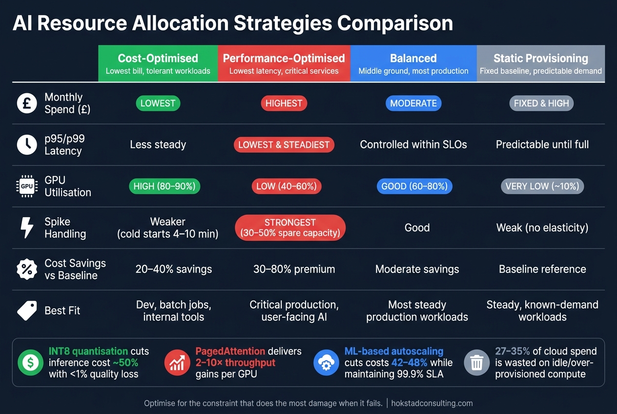 {AI Resource Allocation Strategies: Cost vs. Performance Comparison}
:::
{AI Resource Allocation Strategies: Cost vs. Performance Comparison}
:::
How Does AI Optimize Cloud Resource Allocation? - Cloud Stack Studio
Quick comparison
| Approach | Monthly spend | Latency | Throughput | Utilisation | Spike handling | Best fit |
|---|---|---|---|---|---|---|
| Cost-optimised | Lowest | Less steady | Good per £ spent | High | Weaker | Dev, batch jobs, internal tools |
| Performance-optimised | Highest | Lowest and steadier | Highest | Lower | Strongest | Critical production, user-facing AI |
| Balanced | Mid-range | Controlled within SLOs | High | Good | Good | Most steady production workloads |
| Static provisioning | Fixed, often high | Predictable until full | Stable but capped | Low | Weak | Steady workloads with known demand |
What matters most is not just cost or speed on its own. I’d judge each model by the same five checks: monthly cost (£), p95/p99 latency, throughput, CPU/GPU/memory use, and how well it handles spikes.
If you run UK-based AI services, the choice often comes down to this: do you want the lowest workable bill, the steadiest user experience, or a middle ground that stays inside your targets?
1. Cost-optimised AI allocation
Cost-optimised allocation cuts spend by using smaller models, lower precision, and as little idle capacity as possible. The goal is simple: hit the lowest workable cost while still meeting an agreed service level.
Infrastructure spend
AWS Inferentia Inf1 instances can deliver up to 2.3× higher throughput and 70% lower cost per inference than similar GPU-based EC2 instances for computer vision workloads.[1][2]
On the software side, INT8 quantisation can cut inference cost by about 50% with less than 1% quality loss. Continuous batching can also cut GPU cost by about 50%, though it usually comes with roughly 20% higher latency.[11]
There are also some plain, practical savings that add up fast:
- Shut down non-production environments outside working hours
- Rightsize GPU instances instead of paying for more than you use
- Stack software gains with infrastructure changes to cut spend further
Latency and throughput
Batching lowers the cost per inference, but it usually adds 20% or more latency.[5][11] For internal tools, that’s often a fair trade. Think document summarisation, batch analysis, or overnight reporting. A short delay there usually doesn’t hurt.
For customer-facing assistants, it’s a different story. If users are waiting on replies, response time shapes the whole experience. In that setting, cheaper isn’t always better.
The main throughput gains in this setup come from batching and queueing rather than peak capacity. So the measure that matters is efficiency per pound spent, not raw top-end speed.
Utilisation efficiency
Many organisations run GPUs at only 20–40% average utilisation, which means a big slice of GPU spend goes to waste.[3][9][12] Cost-optimised allocation deals with that by consolidating workloads and using shared inference pools. The idea is to pack multiple services onto as few nodes as possible.
One documented example shows 21 inference services running on three A100 GPUs, cutting node count without sacrificing throughput.[13] On top of that, elastic autoscaling alone typically delivers a 15–30% cost reduction by cutting idle GPU time.[3]
Scaling stability
Spot capacity and tightly packed nodes can struggle during sudden demand spikes, which can lead to queue backlogs.[4][5][6][8][10] To keep things steady, tune autoscaling against queue depth or SLO measures such as p95/p99 latency or time-to-first-token. Keep a small baseline buffer in place, and delay scale-down so the system doesn’t bounce up and down.
This setup works best when workloads are predictable or can handle short delays. It’s a poor fit when steady sub-second response times are non-negotiable.
When latency or service-level targets tighten, the next move is to add a steadier baseline without giving up all the savings.
2. Performance-optimised AI allocation
After cost-first allocation, the next challenge is different: keeping latency low and reliability steady when demand jumps. Cost-optimised allocation asks, how little can we spend? Performance-optimised allocation asks, what does it take to keep the user experience strong, all the time? That usually means a higher baseline spend, but not without reason.
Infrastructure spend
Performance-optimised setups are built for peak load. That means larger GPU instances, more replicas and, for UK users, nearby clusters in London or Dublin. Keeping workloads close can cut 20–50 ms from end-to-end latency compared with regions farther away.[19][20][21]
The trade-off is simple: more fixed spend each month. Organisations that over-provision for performance often end up with 20–40% higher infrastructure costs than cost-optimised baselines.[19][20][21] Autoscaling helps trim idle spend, so use it where it makes sense.
One thing you shouldn't do is scale interactive LLMs to zero. Cold starts on serverless GPU instances can add 5–30 seconds of delay, and for very large models that can stretch into several minutes.[14][18][21] For user-facing systems, that's painful. Keep at least one warm replica running in each region, and treat that standing cost as part of the plan rather than an afterthought.
Latency and throughput
The aim here is steady, predictable response times. Dedicated GPUs with preloaded models can deliver under 100 ms first-token latency for LLMs. Serverless setups can hit similar numbers too, but only when they're already warm.[14][15][16][19][20][21] In production, interactive AI workloads often target median latencies below 200–300 ms for standard inference, while keeping p95 latency within two to three times the median.[19][20][21]
Throughput comes from tuning the whole serving path, not just adding more hardware. Continuous batching, multiple model replicas and traffic sharding all help. Techniques such as PagedAttention can deliver 2–10× throughput improvements and support 2–4× more concurrent requests per GPU for LLM serving.[22][23][24]
A good example is Uber's Michelangelo prediction platform, which handles 1 million queries per second across the platform with a p95 latency of 5–10 ms.[25][26][27] Numbers like that don't come from one trick. They come from tuning the model, the serving stack and the hardware together.
Utilisation efficiency
Higher provisioning doesn't automatically mean money is being wasted. The target isn't maximum GPU utilisation at all costs. It's the best balance between latency and throughput.
One approach that stands out is operator-level autoscaling, where individual pipeline stages scale instead of full replicas. Research on this method, called OpScale, found that it can keep latency SLOs in check while using up to 36.3% fewer GPUs and 28% less power. Under a fixed budget, it can also deliver 44% higher throughput.[17] That's the kind of gain teams want: lower spend pressure without giving up the performance guarantees that made this setup worth choosing.
Scaling stability
Critical clusters should keep 30–50% spare capacity so they can absorb spikes without queues building up, especially during releases and traffic surges. In the UK, seasonal peaks such as Black Friday and end-of-year tax submission periods often push teams to lift baseline capacity for a while and tighten autoscaling thresholds. Yes, that can mean a short-term cost increase, but it's often the safer call when reliability is on the line.
Rolling deployments and canary releases also help by reducing the chance that a model update brings a latency regression during a busy period. The biggest stability risk is over-aggressive autoscaling. If scale-up happens too fast, you can hit quotas. If scale-down happens too fast, you end up with oscillation.
When that amount of headroom costs too much, the balanced model sits in the middle.
3. Balanced AI allocation
Balanced AI allocation is about keeping cost and latency inside your SLOs without swinging too far in either direction. The usual setup is simple: keep a reserved baseline for day-to-day demand, then add autoscaled capacity when traffic spikes. The hard part is finding that middle ground so you’re not paying for idle capacity or falling short when demand jumps.
Infrastructure spend
A balanced setup blends committed capacity with flexible capacity so spend stays within a target range, while still leaving room for peaks. In practice, that often means using spot or pre-emptible instances for batch inference jobs that can wait a little, right-sizing models and instances, and making scaling decisions based on SLOs, queue depth, and tail latency.
This works best when teams stop treating raw utilisation as the main signal. A service can look busy on paper and still miss response targets. Machine-learning-based autoscaling has cut operational costs by 42–48% while maintaining above 99.9% SLAs.[30]
Latency and throughput
Balanced allocation aims for steady latency within agreed limits, not the lowest latency at any price. That’s a big difference. If you optimise only for speed, costs can climb fast.
A better approach is to scale on queue depth, tokens per second, and tail latency rather than raw GPU utilisation. Continuous batching is a good example of why. It can push GPU utilisation from about 15–30% up to 60–80%, which leads to 3–4× higher effective throughput at the same infrastructure cost for LLM inference.[28]
Utilisation efficiency
For a balanced strategy, the usual target band is 60–80% utilisation. That’s high enough to avoid waste, but low enough to give you breathing room when short bursts hit.[9]
If GPU utilisation stays below 30%, that’s usually a sign of overprovisioning. At that point, teams can trim instance size, increase batching, or run more concurrent models on the same GPU. Continuous batching, quantisation, and multi-model serving on shared GPUs all help squeeze more work out of each £ spent.[7][28][29]
Scaling stability
Balanced allocation also reduces the risk of the stop-start behaviour that comes with aggressive autoscaling. If capacity drops too fast and traffic returns, systems can stumble. That’s why teams set cooldown periods on scale-down, use predictive or scheduled scaling for known demand patterns, and place fixed minimum and maximum limits on each service.
Known patterns matter here. Weekday-versus-weekend shifts are common, and retail traffic around Black Friday or Christmas can be sharp enough to punish a poor scaling policy. A reserved baseline handles normal demand, while autoscaling picks up the surges. Too little headroom leads to throttling or OOM errors during recovery. Too much headroom means expensive GPUs sitting idle.
When that balance is removed entirely, the model becomes fixed provisioning.
4. Static provisioning baseline
At the other end of the spectrum, static provisioning removes elasticity entirely. You keep a fixed pool of compute running whether demand is high, low, or barely there at all. It’s the control case: simple, predictable, and rigid.
Infrastructure spend
Static capacity is usually sized for peak demand, or close to it. That means you’re paying for spare headroom 24/7. In UK cloud setups, that turns into a steady monthly bill in £, with money tied up in capacity that often sits idle.
Industry surveys keep landing on the same point: around 27–35% of cloud spend is wasted, and idle or overprovisioned compute is one of the main reasons.[34][35][36] For AI workloads, the problem can bite harder. GPU instances are expensive, and if they sit underused for long stretches, the effective cost per inference or training job climbs fast. Shifting inference workloads from always-on static capacity to autoscaled setups can cut costs by 20–40%.[33] For workloads with steady demand, reserved or committed-use discounts can still make static provisioning workable.
Latency and throughput
Static provisioning does have one clear upside: predictable latency. The capacity is already there, so you don’t get cold starts or autoscaling lag. Throughput stays steady too, right up until demand pushes past the fixed limit.
That makes this model a good fit for latency-sensitive services such as fraud detection and other real-time inference workloads where immediate responses matter. The downside shows up when demand goes beyond the baseline. Once that happens, the system hits a hard ceiling, and latency and error rates can climb because no extra nodes are added on their own.
Utilisation efficiency
This is usually where static provisioning falls short. Kubernetes benchmarks have found average CPU utilisation as low as 10%, which means roughly 90% of capacity can sit idle.[31][32]
Teams can trim some of that waste by sizing headroom from observed data instead of broad safety buffers. A common approach is P95 usage plus 20%.[37][38] Where fixed capacity can’t be avoided, a few practical steps help:
- periodic rightsizing
- workload consolidation
- off-peak batch scheduling
None of that removes the core issue, but it can claw back some unused capacity.
Scaling stability
Static provisioning is stable by design. Capacity stays the same over time, so there’s no autoscaler moving things up and down, less day-to-day churn, and monitoring thresholds and runbooks tend to stay valid for longer. Disaster recovery planning is simpler too, because the capacity in each region is known in advance and fixed.
The catch is plain enough: there is no elasticity. If demand grows beyond the baseline, the only option is manual intervention.
The deciding factor is how often demand moves beyond the fixed baseline.
How the right strategy depends on your deployment environment
No single allocation strategy works in every setup. The right pick comes down to workload, SLOs, and how much failure you can live with. The simplest way to use these models is to map them to the deployment environment.
Development should lean hard towards cost control. Teams can usually live with slower response times and the odd interruption. That makes spot instances, mid-range GPUs, and heavy overnight scale-down perfectly reasonable. For example, you might power clusters down from 18:00 to 08:00 UK time and save a fair bit without causing much pain.
Test and staging sit somewhere in the middle. They need to act enough like production to give you results you can trust, but they don't need production-level spend. A balanced setup works well here: representative instance types, scheduled scaling, and budget caps on concurrent jobs. You keep spend under control without ending up with test data that tells the wrong story.
Production is where the trade-off changes, especially for customer-facing AI services like recommendation engines or conversational agents. These systems need low and predictable latency. For interactive services, example SLOs are 90% of requests under 100 ms and 99% under 900 ms[39][40]. When users feel the delay, performance matters more than utilisation. It's worth paying a higher baseline, but only for services that are both user-facing and latency-sensitive. Internal production workloads, such as batch analytics or offline scoring, don't always need that treatment. In those cases, a balanced setup can work well, with cost controls applied where latency isn't visible to users.
Hybrid cloud adds another wrinkle. Here, placement matters just as much as scaling. A static or balanced baseline on-prem helps you get more from hardware you already own, while public cloud capacity handles bursts. Data-local workloads should stay where latency needs and UK GDPR demand it. In other words, allocation isn't just about traffic shape. It's also about data locality and hardware ownership. AI inference close to user traffic often fits the cloud better, while training and batch scoring can stay on-prem where utilisation is higher and marginal cost is lower.
AI-heavy burst workloads need their own default. Think Black Friday recommendation spikes or a scheduled large-scale model retraining window. Static provisioning on its own is a poor fit here. If you size for peak all year, you end up paying for idle capacity most of the time. A better pattern is a static baseline for normal demand, then performance-focused capacity for peaks. Research on burst-aware autoscaling found a 57% average drop in SLO violations and a 10% cut in resource costs compared with other autoscaling methods[41]. For internal training bursts, cost-led spot capacity with flexible scheduling is often enough. That's the key point: burst workloads should not be treated like steady-state workloads.
The table below shows the default fit by environment.
| Environment | Recommended Strategy | Cost Pressure (£) | Latency Target | Utilisation Target | Failure Tolerance |
|---|---|---|---|---|---|
| Development | Cost-optimised | High | Seconds to minutes | 80–90% | High - outages acceptable |
| Test / Staging | Balanced | Medium | Seconds | 75–85% | Medium - release delays acceptable |
| Production (critical) | Performance-optimised | Low | Sub-second | 40–60% | Very low - customer impact unacceptable |
| Production (internal) | Balanced | Medium | 1–3 seconds | 70–75% | Low |
| Hybrid Cloud | Balanced with static baseline | Mixed | Depends on data locality | 60–70% on-prem | Medium - depends on failover design |
| AI-Heavy Burst | Performance-optimised | Elevated during bursts | Sub-second | High during burst window | Low for revenue-critical; medium for internal |
Pros and cons of each allocation approach
The table below gives a side-by-side look at the four models across cost, speed, resilience and waste.
| Approach | Monthly spend (£) | Throughput | Resilience | Utilisation | Key Risk |
|---|---|---|---|---|---|
| Cost-optimised | Lowest | Variable; throttling is possible | Moderate; spot capacity can be reclaimed | High | Under-provisioning during spikes |
| Performance-optimised | Highest | Highest; spare capacity is always available | Highest; spare capacity and multi-zone spread | Low | Overspend and idle capacity |
| Balanced | Moderate | High for critical paths | High for critical paths | Good | Scaling lag during unexpected surges |
| Static provisioning | Fixed and high | Stable but capped | Weak; fixed capacity only | Very low | Persistent waste and limited flexibility |
The contrast stands out most when you look at how each model fails under pressure.
Cost-optimised is the cheapest route, but that lower bill comes with real trade-offs. Autoscaling rules set up to save money can introduce a cold-start delay of around 4–10 minutes from trigger to fully warmed instances[42]. During that gap, 10–30% of requests can see higher latency or even fail[42]. That makes it a decent fit for batch jobs and internal tools, but a poor choice for user-facing services where delays are hard to hide.
Performance-optimised goes in the other direction. It cuts much of that risk by keeping spare capacity ready all the time. The catch is cost. Fixed headroom and premium instance types can lift monthly bills to 30–80% above a cost-optimised baseline, while average GPU utilisation often falls below 40% outside peak times. It makes sense when downtime costs more than extra capacity. If not, you're paying for machines that mostly sit there, and that bill adds up fast.
Balanced sits in the middle. Spend stays moderate, while SLA protection remains strong. But this model only works well if your forecasts are good. If demand estimates are off, or observability is weak, the setup can drift into overspend or under-provisioning without much warning. In practice, observability and forecasting are the guard rails here.
Static provisioning is the easiest model to run and usually the easiest to budget for as well. The problem is simple: fixed capacity means fixed waste when demand drops. It tends to work best as a baseline layer under autoscaling, not as a model on its own.
Conclusion
Taken together, these four models point to a simple rule: optimise for the constraint that does the most damage when it fails. Cost and performance pull in different directions. The right model is the one that fits your workload, SLOs, and tolerance for failure, judged against the same measures used throughout this article: monthly cost, p95/p99 latency, throughput, utilisation, and spike resilience.
In practice, the best fit usually looks like this: static provisioning works for predictable, low-risk jobs; cost-optimised allocation fits tolerant internal workloads; balanced allocation fits most steady production services; performance-optimised allocation fits latency-critical systems.
That choice shouldn’t stay fixed. Workload patterns shift, traffic moves, and risk changes. So allocation needs to be treated as an ongoing operational decision, not a one-off setup.
The aim isn’t to pick the cheapest or fastest model once and call it done. It’s to keep allocation lined up with real demand. If you need to cut cloud and AI infrastructure waste without slowing deployments, Hokstad Consulting can help you find and fix allocation choices that no longer match demand.
FAQs
How do I choose the right allocation model?
Align your allocation model with business goals, workload priority, and data. Put performance-focused settings on critical services. Use cost-focused settings for batch jobs, analytics, and test workloads.
Track both technical metrics, such as p95 latency and throughput, and financial KPIs like cost per 1,000 requests. Start with an audit. Then test changes on non-critical workloads first, using monitoring, automation, and financial guardrails to keep costs under control.
What metrics should I track first?
Start by setting a baseline for your current cloud spend and resource use. That gives you a clear picture of where money is going and which workloads are doing too little with too much.
Then focus on three areas:
- Resource metrics: Track CPU, memory and GPU use to spot over-provisioning. If utilisation sits below 60%, that often points to a rightsizing job.
- Performance metrics: Watch p95 latency, throughput and request rates so your Service Level Objectives stay on track.
- Financial metrics: Review tagged costs by project or model, with close attention on cost per request and cost per prediction.
This mix helps you connect usage, speed and spend instead of looking at each one in isolation.
When should I move away from static provisioning?
Move away from static provisioning when workloads swing a lot over time, like traffic spikes, seasonal peaks, or hard-to-predict demand. Fixed resources often create a lose-lose situation: they either sit idle and waste money, or they come up short and hurt performance.
It also makes sense when you’re seeing steady underuse. For example, if GPU utilisation stays below 60% for a long stretch, that usually points to over-provisioning.
A sensible way to start is with non-critical services. Check the recommendations first, make sure they hold up in practice, and then shift from partial automation to full automation as your confidence builds.