
Rate limiting is essential for managing traffic, protecting infrastructure, and controlling costs in systems that handle high volumes of requests. Without it, sudden traffic spikes can lead to service disruptions, increased expenses, or API misuse. This article breaks down seven rate-limiting algorithms, explaining how they work, their strengths, and their use cases.
Here’s a quick overview of the algorithms covered:
- Token Bucket: Allows bursts of traffic by using tokens that refill at a steady rate. Ideal for handling irregular traffic patterns.
- Leaky Bucket: Smooths traffic by processing requests at a constant rate. Best for preventing backend overload.
- Fixed Window Counter: Tracks requests in fixed time intervals but struggles with boundary spikes.
- Sliding Window Log: Tracks exact timestamps of requests for high accuracy but requires more memory.
- Sliding Window Counter: Combines accuracy and efficiency by smoothing traffic over rolling time windows.
- Generic Cell Rate Algorithm (GCRA): Enforces precise request intervals with minimal memory usage.
- Fixed Window: Simple and efficient but prone to burst issues at interval boundaries.
Each algorithm has unique trade-offs in terms of memory usage, accuracy, and handling of traffic bursts. For most public APIs, the Sliding Window Counter offers a good balance of precision and efficiency. If your system needs to handle sudden traffic spikes, the Token Bucket is a strong choice, while the Leaky Bucket is preferred for steady traffic regulation.
Choosing the right algorithm depends on your specific needs, such as traffic patterns, memory constraints, and the level of precision required. Let’s explore these algorithms in detail to help you make an informed decision.
12. Design Rate Limiter | API Rate Limiter System Design | Rate Limiting Algorithms | Rate Limiter
1. Token Bucket
The Token Bucket algorithm operates like a virtual container that holds tokens, with each token granting permission to process one request. The bucket has a fixed size (b) and refills at a constant rate (r). When a request comes in, it consumes a token. If the bucket is empty, the request is either rejected or placed in a queue [6].
This method is particularly effective for managing bursty traffic while maintaining a consistent output rate. During periods of low activity, tokens accumulate up to the bucket's maximum capacity. This allows the system to handle sudden traffic spikes - such as when a mobile app reconnects - by using the stored tokens to process requests immediately [6]. As Ashish Pratap Singh, Founder of AlgoMaster, explains:
The Token Bucket algorithm is one of the most popular and widely used rate limiting approaches due to its simplicity and effectiveness[7].
Memory Efficiency
One of the standout features of the Token Bucket algorithm is its minimal memory usage. It only requires two data points per user: the current token count and the timestamp of the last refill. This typically equates to about 50 bytes per user [8]. Additionally, the algorithm calculates tokens on-the-fly, eliminating the need for resource-intensive background timers [8]. This efficiency makes it a go-to choice for systems with high user demand.
Handling Bursty Traffic
Many major platforms, such as AWS API Gateway and Stripe, use variations of the Token Bucket algorithm to handle traffic spikes. These systems can be configured with a steady-state rate - like 1,000 requests per second - and a burst capacity of 2,000 tokens. This setup allows them to absorb sudden surges in demand while still enforcing long-term rate limits [2]. This flexibility makes the algorithm particularly well-suited for user-facing APIs where occasional bursts are common.
Precision in Distributed Systems
In large-scale distributed systems, maintaining consistent rate limits across multiple servers can be a challenge. A centralised store, such as Redis, is often used to synchronise limits. Without this coordination, independent servers could unintentionally exceed the allowed rate. Redis operations, like the INCR command, typically take about 0.1 milliseconds, fitting comfortably within most latency budgets. Using Lua scripts ensures the check-and-consume process is atomic, preventing race conditions when handling simultaneous requests [1].
2. Leaky Bucket
The Leaky Bucket algorithm works much like its name suggests - a bucket with a steady drip. Requests come in at irregular intervals, but they’re processed at a constant, predictable rate[9]. This ensures a smooth and consistent output, even when the input traffic is erratic.
There are two main ways to implement this algorithm. The queue-based approach uses a first-in–first-out (FIFO) buffer to hold incoming requests. These requests are processed at a fixed rate, and if the queue fills up, any new requests are simply discarded[10]. On the other hand, the counter-based version, often called a meter
, works by incrementing a counter for each incoming request. This counter is then decremented at a steady rate, much like the Token Bucket algorithm but in reverse[11]. While the Token Bucket allows bursts, the Leaky Bucket ensures a constant flow. As Andrew S. Tanenbaum explains:
The leaky bucket algorithm enforces a rigid output pattern at the average rate, no matter how bursty the \[input\] traffic is[9].
Traffic Smoothing Capability
The Leaky Bucket shines when it comes to smoothing out traffic. For example, Netflix uses a variation of this algorithm to regulate the flow of streaming data, preventing server overloads during peak viewing times[2]. Shopify also applies this concept for its REST Admin API. Users on the Standard plan are given a bucket size of 40 requests with a leak rate of 2 requests per second, while Shopify Plus users enjoy a larger bucket size of 400 requests with a leak rate of 20 requests per second[3]. By maintaining a steady flow, this method protects backend systems from being overwhelmed.
Memory Efficiency
The memory needs of the Leaky Bucket depend on its implementation. The counter-based version, like the Token Bucket, requires about 50 bytes per user[8]. In contrast, the queue-based version demands more - approximately 1KB per user - to store the queued requests[8]. Because of its lighter memory footprint, the counter-based method is often favoured for basic API rate limiting, where the primary goal is to check if a user has exceeded their limit[9].
Suitability for Bursty Traffic
One drawback of the Leaky Bucket is its poor handling of bursty traffic. Unlike the Token Bucket, which can accommodate occasional bursts, the Leaky Bucket drops or delays requests once its capacity is reached[7]. This rigid output can lead to increased latency during traffic spikes, making it less ideal for user-facing APIs. For example, if a mobile app reconnects and tries to sync data, the steady processing rate can slow things down significantly[8].
Next, we’ll look at another approach that offers a different balance of trade-offs for managing rate limits.
3. Fixed Window Counter
The Fixed Window Counter is one of the simplest methods for rate limiting. It works by dividing time into fixed intervals and using a single counter for each interval. Every incoming request increments the counter until it hits a predefined limit, after which it resets at the start of the next interval.
This simplicity, however, comes with a drawback: the boundary spike problem. Requests that fall near the edges of two consecutive intervals can effectively double the rate limit. As Code Experts explain:
Fixed Window is simple but has the boundary spike problem[13].
Despite this limitation, major platforms like GitHub and X still rely on this approach, accepting the trade-off [3].
Memory Efficiency
One of the key advantages of this algorithm is its minimal memory usage. It requires just a single counter per user per interval. To avoid memory leaks, mechanisms like Redis TTL or periodic cleanup tasks are often recommended.
Precision in High-Scale Environments
In horizontally scaled systems, local counters can lead to users exceeding global rate limits due to race conditions. Cloudflare's research highlighted that while Fixed Window counters struggle with boundary issues, their Sliding Window Counter alternative achieved an error rate as low as 0.003% across 400 million requests [3]. For production environments, a fail-open strategy - where requests are allowed if the central counter system fails - can help maintain service availability during outages.
Handling Bursty Traffic
The Fixed Window Counter is not designed to smooth out traffic bursts. Unlike algorithms like Leaky Bucket, it processes all requests immediately until the limit is reached. This can lead to resource exhaustion during sudden spikes. For example, the quota could be consumed within milliseconds, potentially overloading backend systems. To mitigate this, it's common to implement secondary, more granular limits - such as 5 requests per second alongside a 100-per-minute cap. Slack API employs this strategy, using 1-minute fixed windows with tiered limits ranging from 1 to 100 requests per minute.
Next, we’ll dive into approaches that provide better precision and manage bursts more effectively.
4. Sliding Window Log
The Sliding Window Log approach works by keeping a timestamp for every incoming request. When a new request is received, the system removes timestamps that fall outside the current window (e.g., the last 60 seconds). It then counts the remaining timestamps to decide whether the request should be accepted or rejected, based on the defined limit [15][17]. Unlike fixed intervals, this method ensures the window shifts dynamically with each request, maintaining a continuous flow.
That said, the method is memory-intensive. Since it stores one timestamp per request, memory usage increases linearly with traffic volume (O(n) per client) [17][18]. In high-traffic situations, such as a limit of 10,000 requests per hour, the system must handle and store 10,000 timestamps for each user [18]. As William Johnston points out, this makes it inefficient for high-volume scenarios
[18]. Despite its memory demands, the precision of this method is crucial for applications where exact request counts are non-negotiable, paving the way for more memory-friendly alternatives.
Precision in High-Scale Environments
Compared to fixed window methods, which can suffer from boundary issues, the sliding window log avoids the boundary burst
problem. For instance, Cloudflare's analysis of 400 million requests from 270,000 sources reported an error rate as low as 0.003%, with very few threshold violations [16]. This makes it particularly suitable for sensitive applications like payment systems or authentication services, where accuracy takes precedence over memory usage [18].
In distributed systems, tools like Redis Sorted Sets provide an efficient way to implement this method. Commands such as ZREMRANGEBYSCORE (to remove expired timestamps), ZCARD (to count current entries), and ZADD (to log new requests) allow for atomic operations [17][18]. This ensures consistency across servers and eliminates race conditions, all while maintaining precise control.
Memory Efficiency
While this algorithm delivers exact rate-limiting, it comes at the cost of linear memory growth. For public APIs serving millions of users, the overhead of storing and managing logs can strain system resources [15][3]. To mitigate this, it's essential to configure TTLs (time-to-live) on log keys. This ensures that data from inactive users is automatically removed, reducing the risk of memory leaks in production [17][18].
5. Sliding Window Counter
The Sliding Window Counter addresses some of the inefficiencies found in the Sliding Window Log, offering a more streamlined and practical solution.
This method combines the straightforward nature of fixed windows with the accuracy of rolling calculations. It works by maintaining two counters for each user or API key: one for the current window and another for the previous window. When a request comes in, the system calculates an estimated count using the formula:
Estimated Count = Current Window Count + (Previous Window Count × Weight)
The weight is determined by how much of the previous window overlaps with the current one, calculated as:
(Window Size – Elapsed Time in Current Window) / Window Size.
This method effectively resolves the boundary issues seen in fixed window algorithms. As software engineer Chaitanya Srivastav explains:
The Sliding Window Counter was introduced to fix the boundary burst problem of the Fixed Window algorithm... it evaluates requests over a rolling time window, improving fairness[14].
Memory Efficiency
One of the major strengths of this algorithm is its minimal memory usage. It requires only O(1) space, as it stores just two integers per tracking key. This is a stark contrast to the Sliding Window Log, which needs to store every individual request timestamp. Mojtaba (MJ) Michael, a software architect, highlights this trade-off:
The counter version trades a tiny bit of precision for O(1) space - ideal for scale[19].
This efficiency is crucial in distributed systems where scalability is a priority. For example, in environments handling millions of requests, the algorithm is often implemented using Redis. Atomic operations or Lua scripts are employed to manage the check-and-increment process without introducing race conditions.
Precision in High-Scale Environments
In February 2024, Cloudflare tested this algorithm on 400 million requests from 270,000 unique sources. The results were impressive: no false positives were recorded, and only three sources exceeded the rate limit by less than 15%. The average error was just 6%, with an overall error rate of 0.003% [16]. For high-traffic systems, this algorithm achieves an accuracy of 95% to 99%, making it a reliable choice for APIs that demand strict rate limiting without the overhead of tracking every request.
Traffic Smoothing Capability
Unlike fixed window methods that reset abruptly, the Sliding Window Counter continuously calculates a weighted average, which helps to smooth out traffic spikes. For systems with longer time windows, such as hourly or daily limits, grouping requests by minute can maintain a smooth sliding window effect while keeping computational demands low.
In the next section, we'll compare these algorithms to help you determine the best fit for your system.
6. Generic Cell Rate Algorithm (GCRA)
GCRA introduces a method that focuses on using minimal memory while maintaining precise rate control, making it an efficient choice for rate-limiting tasks.
Initially designed for ATM networks, GCRA operates by tracking a single value: the Theoretical Arrival Time (TAT). This value determines when the next request should ideally arrive. When a request is received, GCRA checks if it’s too early by comparing the actual arrival time to the TAT minus a tolerance parameter (τ). If the request passes this check, the TAT is updated. As Tony Finch puts it:
GCRA does the same job as the better-known leaky bucket algorithm, but using half the storage and with much less code[22].
Memory Efficiency
One of GCRA's most appealing features is its minimal memory requirement. Unlike token and leaky bucket algorithms - which need both a counter and a timestamp - GCRA only requires a single timestamp per user. Philip Jones, the maintainer of Quart and Hypercorn, highlights this:
The time-bucket approach requires the storage of two values and does not enforce a rate, while the leaky-bucket approach requires a separate process to continually refill the bucket. In comparison GCRA requires only a single value[24].
This simplicity translates to a 50% reduction in memory usage, making it an excellent choice for high-traffic systems where memory efficiency is critical [22].
Traffic Smoothing Capability
GCRA ensures a consistent flow of requests by enforcing a steady interval between them. It also allows for controlled bursts by adjusting the tolerance parameter (τ). A larger τ allows for more requests in a shorter time, while a smaller τ enforces stricter spacing [21][24]. As Wikipedia explains:
Because there is no simulation of the bucket update, there is no processor load at all when the connection is quiescent[20].
This ability to smooth traffic while remaining efficient makes GCRA a practical choice for managing request rates.
Precision in High-Scale Environments
GCRA calculates its state in real-time upon each request's arrival, avoiding the burst issues seen in fixed window methods [20][23]. However, in distributed systems, clock synchronisation becomes a challenge. Variations in server clocks can lead to false positives. To counter this, using a centralised time source - like Redis's TIME command - can help maintain accuracy [23].
With its precision and low memory demands, GCRA proves to be a strong contender for systems where efficiency and precise rate control are priorities.
7. Fixed Window
Building on the efficiency of GCRA, the Fixed Window approach offers a straightforward solution for scenarios where simplicity and minimal memory usage are key priorities.
This method divides time into discrete, non-overlapping intervals - often 60 seconds long - where each interval has a single counter to track requests. When a request is made, the system checks if the counter is below the allowed limit. If it is, the request is processed, and the counter increases. At the start of the next interval, the counter resets to zero [1].
Unlike the Fixed Window Counter method discussed earlier, this approach strictly adheres to non-overlapping time intervals. Its simplicity makes it incredibly easy to implement. For instance, RD Blog (January 2024) showcased a Java implementation using ConcurrentHashMap and atomic updates. In their example, a request at 0 ms was allowed under a 1 request per 2 seconds limit, but a request at 999 ms was blocked until the counter reset at 2,000 ms [12]. Similarly, GitHub uses this method for its public API, capping unauthenticated traffic at 60 requests per hour with Redis counters that reset hourly [2].
Memory Efficiency
One of the major advantages of the Fixed Window approach is its minimal memory requirement. It only needs a single counter per user (or key) for each time window. Unlike the Sliding Window Log, which must store timestamps for every request, Fixed Window keeps things simple with just one counter per interval [1].
Handling Bursty Traffic
The Fixed Window method does have a notable drawback: the boundary problem.
For example, if a user sends 100 requests at 12:00:59 and another 100 at 12:01:00, they could effectively bypass a limit of 100 requests per minute by doubling their allowable rate. This limitation is acknowledged in real-world API implementations. For instance, Twitter uses a 15-minute fixed window for most endpoints, while Slack employs a 1-minute window with tiered limits ranging from 1 to 100 requests per minute [5]. To address boundary issues, combining larger time windows with more granular limits - like 10 requests per minute alongside 2 requests per second - can help smooth out traffic spikes [5].
Performance in High-Scale Systems
While the Fixed Window approach is simple, its precision in distributing requests within a window is limited. This makes it less accurate compared to other algorithms. However, it compensates with excellent performance. Redis-based setups, for example, can use the INCR command to achieve latencies as low as 0.1 ms [1]. This makes Fixed Window an excellent choice for basic rate-limiting needs, such as managing free-tier API usage or restricting login attempts, where absolute precision is less critical than maintaining system performance [2].
Algorithm Comparison
::: @figure 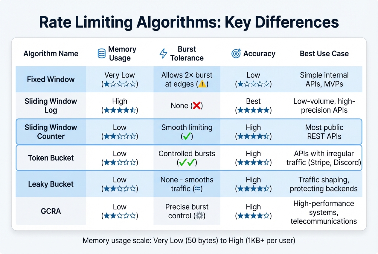 {Rate Limiting Algorithms Comparison: Memory, Accuracy, and Burst Handling}
:::
{Rate Limiting Algorithms Comparison: Memory, Accuracy, and Burst Handling}
:::
Selecting the right rate limiting algorithm hinges on understanding your traffic patterns and the specific needs of your system. Each algorithm comes with its own strengths and trade-offs, particularly in terms of memory usage, accuracy, and how well it handles traffic bursts. Here's a breakdown of the key options to help you decide.
The Sliding Window Counter strikes a balance between accuracy and efficient memory usage, making it a popular choice for most production APIs. It’s particularly suited for modern REST APIs that need steady rate limiting without consuming too many resources.
If your system deals with bursty traffic, the Token Bucket algorithm stands out. For instance, Stripe uses this approach to allow up to 25 requests per second, while Discord enforces a global limit of 50 requests per second[3].
For scenarios where downstream systems need protection from sudden traffic spikes, the Leaky Bucket algorithm is a great fit. Shopify implements this method in its REST Admin API, with standard plans limiting the bucket to 40 requests and a leak rate of 2 requests per second. Shopify Plus customers benefit from increased limits, with a bucket size of 400 and a leak rate of 20 requests per second[3].
Here’s a comparison table summarising the strengths and use cases of each algorithm:
| Algorithm | Memory Usage | Burst Tolerance | Accuracy | Best For |
|---|---|---|---|---|
| Fixed Window | Very Low | Allows 2× burst at edges | Low | Simple internal APIs, MVPs |
| Sliding Window Log | High | None | Best | Low-volume, high-precision APIs |
| Sliding Window Counter | Low | Smooth limiting | High | Most public REST APIs |
| Token Bucket | Low | Controlled bursts | High | APIs with irregular traffic (e.g. Stripe, Discord) |
| Leaky Bucket | Low | None (smooths traffic) | High | Traffic shaping, protecting backends |
| GCRA | Low | Precise burst control | High | High-performance systems, telecommunications |
This table provides a clear snapshot of the differences, helping you identify the best algorithm for your API’s needs.
Conclusion
Picking the right rate limiting algorithm is a critical decision that impacts system stability, cost management, and overall user satisfaction.
Rate limiting isn't optional. It's a core component of any production system.– System Design Sandbox [1]
A 2024 study from Stanford revealed that 68% of public APIs implement rate limiting incorrectly, leading to issues like blocking legitimate users or failing to prevent misuse [4].
Without effective rate limiting, you risk more than just unhappy users. Problems like cascading system failures, skyrocketing cloud expenses, and depleted third-party API quotas can quickly spiral out of control. The algorithm you choose plays a significant role in managing traffic bursts while protecting downstream services from overload.
To avoid these pitfalls, it's important to select an algorithm that balances precision with resource efficiency. For most modern REST APIs, the Sliding Window Counter strikes this balance well. If your app sees unpredictable traffic spikes, the Token Bucket is excellent for managing bursts. Meanwhile, backend systems needing steady traffic flow should consider the Leaky Bucket for its smooth processing capabilities.
Implementation, however, is just as important as the choice of algorithm. In distributed systems, tools like Redis can help manage centralised state efficiently, and using atomic operations prevents race conditions. Aim for your rate limiter to respond in under 20 milliseconds to preserve a seamless user experience. Always return proper HTTP 429 responses with Retry-After headers to guide users effectively [1].
If you're planning to implement or refine your rate limiting strategy, Hokstad Consulting offers expertise in DevOps and cloud cost management, helping you protect resources while maintaining a top-notch user experience.
FAQs
How do I choose the right rate limiting algorithm for my API?
To determine the best rate limiting algorithm, think about what your system needs in terms of handling bursts, maintaining accuracy, managing complexity, and conserving resources.
Token Bucket: Great for allowing bursts and is relatively simple to implement. If your system needs to handle occasional traffic spikes without overloading, this is a strong choice.
Sliding Window: If strict rate enforcement is your priority, this algorithm is highly accurate. However, it does demand more resources to function effectively.
Fixed Window: This method is straightforward and works well for basic scenarios. However, it’s less precise, so it’s not ideal for situations requiring fine-tuned control.
Ultimately, it’s about finding the right balance between fairness for users and your system’s capacity to handle traffic.
What’s the best way to do rate limiting across multiple servers?
When managing rate limiting across multiple servers, distributed algorithms like the Token Bucket or Sliding Window are your best bet. These methods work by sharing counters across servers via a central data store, such as Redis, ensuring fairness and consistency in enforcing limits. To maintain scalability and accuracy, it's crucial to use atomic operations (like Lua scripts) to avoid race conditions and keep all servers in sync.
What should my API return when a client is rate limited?
When a client hits the rate limit, your API should respond with an error message indicating that the limit has been exceeded. This is usually done using the 429 Too Many Requests status code. To improve clarity, you can also include details about when the client can attempt their next request. Providing this information ensures smoother communication and helps clients manage rate limits more effectively.