
If I cut node headroom too far, I may save £400–£600 per month on a mid-sized cluster - but I also make spike-related slowdowns and pending pods more likely. That is the core trade-off.
If I boil this article down to one decision, it is this: I should match each workload to the right node pool policy instead of forcing one setting across the whole cluster. In simple terms:
- Conservative autoscaling trims spend, but leaves less room for traffic jumps.
- Aggressive headroom costs more, but keeps user-facing services steadier under burst load.
- Spot-focused pools can slash compute spend by 60–90%, but nodes may disappear with little warning.
- Bin-packing cuts idle capacity, but can increase noisy-neighbour issues and scheduling delays.
- Multi-pool autoscaling gives me the best fit across mixed workloads, but adds setup and policy overhead.
I also need to keep one fact in mind: new nodes often take 1–3 minutes to come online. So if pods scale out before nodes are ready, users can feel that gap as latency, timeouts, or failed requests.
Quick comparison
| Policy | Cost | Performance under spikes | Best for | Main downside |
|---|---|---|---|---|
| Conservative high-utilisation | Low | Weaker | Batch, internal tools | Less spare capacity |
| Aggressive headroom | Higher | Stronger | Customer-facing apps | More idle spend |
| Spot-focused | Lowest when available | Mixed | ETL, CI/CD, batch | Interruptions |
| Bin-packing | Low to mid | Mixed | Steady workloads | Contention on dense nodes |
| Multi-pool | Varies | Best fit by workload | Mixed estates | More setup and control rules |
If I am choosing between cost and performance, the short answer is simple: pay for headroom where latency matters, and save money where interruption and delay are acceptable.
::: @figure 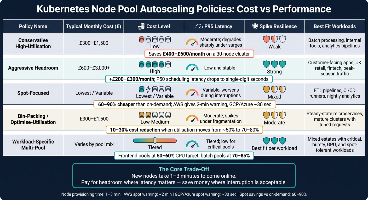 {Kubernetes Node Pool Autoscaling Policies: Cost vs Performance Comparison}
:::
{Kubernetes Node Pool Autoscaling Policies: Cost vs Performance Comparison}
:::
1. Conservative autoscaling with high utilisation targets
This sits at the low-cost end of the range. Conservative autoscaling keeps spare capacity tight, so scale-out tends to happen only when utilisation is already high. In practice, that often means HPA targets around 70–85%, low minimum node counts, and aggressive scale-down settings.
On GKE, this lines up with the optimize-utilization autoscaling profile, which packs workloads onto fewer nodes and scales down hard. On EKS and AKS, you get much the same result through cautious autoscaler settings and tightly right-sized pod requests. That last part matters more than many teams expect. The Cluster Autoscaler scales from pod requests, so padded or inaccurate requests eat into the savings.
This policy fits batch processing, analytics pipelines, scheduled reporting, and internal tooling. These are the kinds of workloads where some latency variation is fine and demand tends to follow predictable UK business calendars.
Monthly cost
Take a production cluster running 30 general-purpose nodes at roughly 45–50% average utilisation, with a monthly cost of about £2,400. Under conservative autoscaling, that can drop to 22–24 nodes with 75–80% targets on non-critical services. That works out to around £400–£600 per month in savings.
The gains stack up when you pair this with request right-sizing. Tighter requests let the Cluster Autoscaler fit more pods onto each node and remove underused nodes sooner.
Latency under load
There’s a trade-off. Under sustained load, median and p95 latency usually climb once utilisation moves past 70–80%. For user-facing services, that means SLO monitoring needs to be tight, especially during weekday business hours when UK traffic is at its peak.
Resilience to spikes
This is the weak spot. Sudden, unplanned spikes are harder to absorb when there’s very little headroom sitting idle. A flash sale or deadline-led traffic jump can push nodes to 90–100% utilisation before the autoscaler has time to react.
New node provisioning usually takes 1–3 minutes, depending on the provider and region. During that window, the cluster can sit in a saturated state, which puts user-facing services at risk of SLO breaches.
Teams often soften this with a couple of simple moves:
- Add scheduled scale-up windows around known UK campaign times
- Set slightly lower utilisation targets, around 65–70%, on customer-facing node pools
- Let batch pools run closer to 80–85%
Operational risk
Running nodes this hot leaves very little room for background work. Jobs that share the same CPU and memory can start competing fast. In multi-tenant clusters, one service’s surprise resource spike can spill over into others almost straight away.
Deployments get riskier too. Even a small performance regression can push utilisation over the limit and trigger SLO breaches on user-facing services. Common safeguards include blue/green or canary rollouts with automatic rollback, along with per-service SLO dashboards set to Europe/London time.
The next policy gives back some of these savings in exchange for more headroom and a faster response to spikes.
2. Aggressive autoscaling with reserved headroom
This policy keeps spare scheduling capacity ready for sudden traffic spikes. It's the opposite of conservative autoscaling.
Instead of waiting for CPU to hit 70–80% before adding capacity, an aggressive setup starts scaling out at around 40–60% utilisation. It also keeps a small amount of spare scheduling capacity available at all times. In practice, that usually means higher minimum node counts, often 1–2 extra nodes per pool above current demand, along with faster scale-up and slower scale-down. Scale-down windows typically sit at 20–30 minutes. HPA thresholds are kept low enough that pods start scaling before nodes come under pressure, so new pods can schedule straight away while extra nodes boot in the background.
Monthly cost
Against a conservative policy at the same average load, aggressive headroom will usually push monthly spend up by 10–40%.
That might mean an extra £200–£300 per month for much lower p95 latency and better burst resilience. For many teams, that is not just extra overhead. It's a cost worth weighing against revenue per request or booking value. In plain terms, the extra spend buys lower queueing and steadier p95 latency.
Latency under load
Keeping utilisation around 50–60% leaves spare CPU ready when traffic jumps. That helps keep request queues short and makes p95 latency less erratic.
Google's buffer tests show how big the gap can be. Without reserved capacity, P50–P99 scheduling latency stayed at 4–6 minutes under the same traffic load. With buffers in place, P50 dropped to single-digit seconds and P95/P99 only briefly peaked at around one minute before settling back [4].
That difference matters most for CPU- and network-bound workloads, like checkout services or ticketing platforms. Those are the moments when demand spikes at the exact time users have the least patience for delay. This policy is at its best when bursts arrive faster than nodes can scale.
Resilience to spikes
This is the main upside.
Pre-allocated headroom takes the first hit of a traffic spike while the Cluster Autoscaler brings up more nodes. Even in ideal conditions, that process usually takes 1–2 minutes [3]. For UK-style traffic patterns such as a Boxing Day sale, a Premier League kick-off, or a concert ticket release, that short window is often where the worst damage happens.
The buffer gives the system breathing room during the first phase of a surge and delays the need for new nodes during a longer spike. That cuts the risk of timeouts and throttling.
Operational risk
The biggest risk is cost drift.
Teams can slowly push minimum node counts upward to patch performance issues. If no one reviews those settings, spare headroom quietly turns into a bigger monthly bill. Put hard maximum node counts in place for each pool, and set monthly budget alerts in £ to keep that drift under control.
It's also worth being blunt about what this policy can't do. Reserved capacity will not fix database limits, cache pressure, or third-party API bottlenecks. If those parts of the stack are the problem, the spare capacity just sits there while users still get slow responses.
This approach fits latency-sensitive, user-facing services where burst risk matters more than the cost of unused capacity. The next approach cuts spend further, but only by taking on more scheduling risk.
3. Spot-focused node pool autoscaling
Run stateless workloads on spot instances, and keep a smaller on-demand pool for the services you can't afford to disrupt. Set the autoscaler to try spot first, then move to on-demand only if spot capacity disappears or gets reclaimed. That's the basic trade-off: lower VM prices in exchange for a higher chance of interruption.
If keeping spare on-demand headroom feels too costly, spot pools can cut spend much further. But they only work well when the workloads are built to handle eviction without much drama.
Monthly cost
AWS, GCP, and Azure all price spot-style instances at 60–90% less than on-demand equivalents.[7][8][10] For a UK SaaS business spending £40,000 per month on compute, shifting 60–70% of stateless workloads to spot at a 70% discount can save around £15,000–£18,000 a month, assuming spot capacity stays available.[7][8][10]
That's a big drop in spend. But there's a catch: those savings depend on interruption events staying rare and on rescheduling happening fast enough that users don't feel it.
Latency under load
The weak point shows up during spot interruptions. When a cloud provider reclaims capacity, pods get evicted and rescheduled onto the nodes that are left. For a short period, CPU usage can jump, and that can trigger p95 and p99 latency spikes until new nodes come up.
AWS provides a 2-minute interruption notice. GCP and Azure give about 30 seconds.[6][7][8] That sounds like a small detail, but it matters. If an endpoint is latency-sensitive, keeping at least one replica on an on-demand node means some serving capacity remains in place even if a spot zone disappears.[7][9]
So the main reliability controls aren't fancy autoscaling settings on their own. They're capacity diversity and fallback placement.
Resilience to spikes
This setup stands or falls on one thing: whether spot capacity is there when demand jumps.
If spot capacity is available, the autoscaler can take the extra load. If it isn't, pods start queueing and error rates climb. A simple way to cut that risk is to spread the spot pool across:
- Multiple instance types
- Multiple availability zones
That gives the autoscaler more than one pool of capacity to draw from when a single pool runs dry.[2][5][7]
For known peaks, like a seasonal promotion, it's far safer to pre-warm both the spot and on-demand baselines ahead of time than to react once the spike has already started. At that point, the main risk isn't the spot model by itself. It's whether workloads have been separated tightly enough.
Operational risk
This is where small mistakes turn into painful outages. A bad affinity rule or a missing taint can place a payment service or authentication component onto a node that may vanish with 30 seconds' notice.
The guardrails need to be strict:
- Use node taints and tolerations properly
- Enforce PodDisruptionBudgets so all replicas of a service aren't evicted at once
- Keep termination grace periods at 30 seconds or less for spot workloads, so pods can shut down cleanly inside the interruption window[6][9]
Watch spot interruptions, unschedulable pods, and scale-up times as the main warning signs. Spot only suits workloads that can survive eviction. The cost savings come from that discipline, not from the instance type alone.
4. Bin-packing and optimise-utilisation policies
Bin-packing takes the opposite approach to spare headroom. Instead of spreading pods out, the scheduler tries to place them on as few nodes as possible. It fills one node, then moves to the next. The result is a smaller, denser fleet.
That usually means lower spend, because you’re running fewer machines. The trade-off is simple: you save money by accepting more contention.
In Kubernetes, placement can be nudged with NodeResourcesFit scoring strategies such as MostAllocated and RequestedToCapacityRatio, which favour nodes that are already heavily used.[11][7] Autoscalers with consolidation support push this further by removing underused nodes and keeping the cluster compact.
Monthly cost
Case studies report 10–30% cost cuts when utilisation moves from about 50% to 70–80%.[14][15][16]
The main lever here is getting pod resource requests and limits right. If requests are too high, the scheduler assumes nodes are fuller than they are. That blocks consolidation and leaves extra nodes running for no good reason.[12][15] In practice, many teams target around 70–80% average CPU utilisation on bin-packed pools. That’s dense enough to trim spend, while still leaving some room for short bursts before scale-out kicks in.[13][15][14]
Latency under load
This is where the downside shows up. Dense packing increases noisy-neighbour risk. When lots of pods share one node, CPU throttling and memory pressure can push up p95 and p99 latency, even when average latency still looks fine. That matters even more for services with synchronous call chains, where contention in one hop can ripple through the whole request path.
For latency-sensitive workloads, it helps to keep 20–25% memory headroom and use Guaranteed QoS settings, where requests equal limits, to cut the risk of eviction under pressure.[13]
Resilience to spikes
Bin-packing leaves less slack for sudden traffic spikes. When demand jumps, the autoscaler has to provision new nodes first and only then schedule pods onto them. That gap can mean a few minutes of slower scheduling and more errors.
For known peak periods, pre-warming nodes can help. Another option is to relax consolidation thresholds for a while, so you don’t get caught by a cold-start gap.
Operational risk
A node failure hurts more in a dense setup because more pods are sitting on that node. In plain terms, the blast radius is bigger. That’s why Pod Disruption Budgets and topology spread constraints matter more when you’re packing nodes hard.[13]
Regular load testing also matters here. So does per-node utilisation monitoring in Prometheus and Grafana. Those checks help teams spot mismatched requests, limits, or packing rules before they turn into outages.
Bin-packing works best when used with care, not everywhere at once. It tends to suit:
- batch processing
- CI/CD runners
- data transformation jobs
- internal tooling
Customer-facing APIs are often better on pools with more conservative headroom. In mixed-criticality clusters, separate pools are usually a better choice than one dense fleet.
5. Workload-specific multi-pool autoscaling
Workload-specific multi-pool autoscaling lets you apply different scaling rules to different workloads, so each service gets the spend level and spare capacity it needs. Instead of forcing one policy across the whole cluster, you run the earlier approaches - conservative, aggressive and Spot-backed - side by side in separate pools in the same cluster. The gain here is simple: not a new scaling method, but a better match between each workload and the policy behind it.
To make this work, you need clear placement rules. Use taints, tolerations, selectors and affinity rules to keep each workload on its intended pool. If you don't, the autoscaler may scale the wrong pool - or fail to scale the right one at all.[17][18][22]
Monthly cost
The cost win comes from stopping one pool from carrying every workload. You cut spend by matching instance type, scaling threshold and pricing model to each workload class. That means one cluster can run conservative pools for internal tooling, aggressive pools for customer-facing APIs and Spot-backed pools for batch jobs, with each one tuned on its own terms.
The main levers are:
- Mixing on-demand and Spot capacity
- Setting different utilisation targets for each pool
- Using time-based scaling for workloads that follow business hours
For example, frontend pools might target 50–60% average CPU to keep headroom in reserve. Batch pools can run harder, at 70–85%. And if a pool only supports office-hours traffic, time-based scaling can trim it outside 09:00–17:30, which helps avoid wasting money overnight.
Latency under load
This same separation also cuts contention. When workloads sit in separate pools, batch jobs, ML tasks and customer-facing traffic stop fighting over the same nodes. That matters when demand jumps and every millisecond starts to count.
For latency-sensitive pools, it often makes more sense to scale at 50–60% rather than 75–80%. CPU on its own doesn't always tell the whole story either. p95 latency or request rate can track user-facing performance more closely than CPU alone.[21]
Resilience to spikes
Isolation also reduces blast radius when traffic surges. Each pool should reflect the spike pattern of the workload it runs. Flash-sale traffic needs higher minimums and shorter cooldowns. ETL jobs are better suited to queue-based scaling. Keeping those in separate pools stops a batch surge from dragging down customer-facing service.
Spot-backed pools need extra care. Keep an on-demand fallback layer in place so pods don't sit pending when Spot capacity disappears.[19][20]
Operational risk
More pools also bring more room for policy drift and placement mistakes. The main failure modes are pretty familiar: latency-sensitive services land on the wrong pool, or the HPA and cluster autoscaler start pushing against each other and create oscillation.
The practical guardrail is infrastructure-as-code. Define node pools, taints, labels and autoscaling policies in version-controlled repositories such as Terraform, Pulumi and Helm. That makes changes easier to review and repeat. It also helps to pair that with shared observability dashboards that show per-pool utilisation and cost next to per-service metrics, so operators can spot how pools and workloads affect each other before a small issue turns into a bigger one.
Cost, Performance and Workload Fit: Policy Trade-offs
Taken together, these five policies mainly differ on three things: cost, p95 latency, and how much interruption your workloads can handle. The trade-off is pretty simple. More headroom usually means better latency and more room for spikes. Tighter packing cuts spend, but it also increases scheduling risk.
Cost tends to climb as headroom climbs. Conservative and bin-packed pools are often the cheapest. Aggressive headroom usually costs more. Spot-backed pools can be the cheapest of all, as long as interruption risk is kept under control.
Latency moves in the same direction. Reserved headroom keeps p95 more stable during bursts. Dense packing and conservative scaling, on the other hand, increase the chance of queueing when demand jumps.
The table below pulls that into one view across workload fit, cost, and risk.
| Policy | Best-fit workloads | Typical monthly cost (£) | Expected p95 latency | Main risk |
|---|---|---|---|---|
| Conservative high-utilisation | Back-office, batch | £300–£1,500 | Moderate; degrades sharply under surges | Scale-up lag; scheduling contention |
| Aggressive headroom | Customer-facing, low-latency | £600–£3,000+ | Low and stable | Idle spend; masks poor workload sizing |
| Spot-focused | ETL, CI/CD, batch | Lowest / variable | Variable; worsens during interruptions | Node eviction with ~2-minute warning |
| Bin-packing / optimise-utilisation | Steady-state microservices | £300–£1,500 | Moderate; spikes under fragmentation | Scheduling contention; noisy-neighbour effects |
| Workload-specific multi-pool | Mixed-criticality estates | Varies by pool mix | Tiered; low for critical pools | Configuration complexity; placement errors |
In practice, the choice comes down to three questions:
- How sensitive is the workload to latency?
- How interruptible is it?
- How predictable is the traffic pattern?
Lower cost usually comes from running with less slack. And less slack usually means slower recovery when traffic spikes.
Latency-sensitive services, such as checkout flows or real-time APIs, are better suited to aggressive headroom or dedicated multi-pool setups. Batch jobs and CI/CD pipelines are a natural match for Spot or conservative policies. AI and ML workloads often split the difference: training runs on Spot to cut spend, while inference sits on reserved capacity for steadier service.
For UK teams dealing with uneven traffic, policy choice and Cluster Autoscaler tuning should be modelled together, not handled as separate calls.
Pros and Cons
This summary turns the earlier comparisons into a quick decision aid. Every policy makes a trade-off between cost and performance. The table below compares cost, latency, resilience, and fit.
| Policy | Key pros | Key cons | Best fit |
|---|---|---|---|
| Conservative autoscaling with high utilisation targets | Lower monthly spend (£); simpler capacity planning; fewer scaling events | Higher utilisation increases the risk of contention and performance degradation under sudden spikes; little spare capacity for unexpected load | Internal tools, batch processing, cost-constrained environments |
| Aggressive autoscaling with reserved headroom | More predictable latency; fast response to traffic surges; better user experience for revenue-critical services | Higher baseline cost (£) because some capacity is kept unused; headroom misconfiguration can cause latency drift | UK retail sites, fintech apps, peak-season traffic |
| Spot-focused node pool autoscaling | Up to 90% lower than on-demand pricing [24]; scales cheaply for batch and CI/CD workloads | Nodes can be reclaimed with as little as two minutes' notice on AWS [2] or 15 seconds on GKE Spot VMs [1]; not suitable for strict SLA workloads unless carefully combined with on-demand pools | ETL pipelines, nightly analytics, CI runners, backup and archiving tasks |
| Bin-packing / optimise-utilisation policies | Reduces idle capacity; improves use of reserved or committed spend; smaller cluster footprint | Dense packing increases contention risk; over-requested pods can block scale-down even when actual CPU usage is low [23] | Mature clusters with well-tuned resource requests and observability |
| Workload-specific multi-pool autoscaling | Fine-grained control per workload; better fault isolation between critical and non-critical services | Higher operational overhead managing multiple pools and policies; misplaced workloads can land on the wrong pool | Mixed estates with critical, bursty, GPU, and spot-tolerant workloads |
In practice, three things usually make the biggest difference: request accuracy, interruption tolerance, and placement control.
Bin-packing works best when requests are accurate. If teams ask for more than they need, scale-down can stall even when actual CPU use stays low [23]. On paper, the cluster looks busy. In reality, it may be carrying spare capacity it cannot shed.
Spot pricing can cut costs hard, and the savings are real. But the trade-off is interruption risk. That means workloads need to handle disruption by design, with checkpointing, retries, PodDisruptionBudgets, and on-demand fallback.
Multi-pool autoscaling can match workloads far more closely, which is often what mixed estates need. But it only works if taints, tolerations, and placement rules are kept under tight control. If those rules drift, workloads can end up in the wrong pool, and the whole setup starts working against you.
Conclusion
There isn't one policy that gives you the lowest cost and the best performance for every workload. The right choice depends on workload volatility, latency and availability needs, and how much capacity your team has to manage it. In practice, this makes the decision less about the platform itself and more about the workload class.
For predictable, throughput-driven workloads, conservative or bin-packing policies usually make sense. For latency-sensitive, user-facing services where burst risk is high, aggressive autoscaling with reserved headroom is often the better fit. Yes, it costs more. But that extra spend can be worth it if it prevents SLA breaches, timeouts and lost conversions.
Spot works well for interruption-tolerant workloads, as long as you put safeguards in place. That includes Pod Disruption Budgets, checkpointing and fallback capacity. Multi-pool setups are a good fit when critical and non-critical workloads need different policies.
Once you know what mix of workloads you're dealing with, separate pools and policies make the trade-offs much easier to control. A staged rollout is usually the simplest path: start with conservative or bin-packing pools, then add headroom for critical services and Spot for batch workloads. If you need help mapping workloads to the right policy mix and putting a £ value on the cost and performance impact, Hokstad Consulting helps UK organisations design and implement staged autoscaling strategies based on measured data.
FAQs
How do I choose the right policy for each workload?
Choose based on whether the workload is stateless or stateful, and on how it uses compute, memory, and node capacity.
For stateless apps like web APIs or microservices, use HPA to scale pods from live metrics. Then use CA when the cluster needs more node capacity to place those extra pods.
For batch jobs or traffic spikes that come out of nowhere, make sure CA and HPA work together. It also helps to set accurate resource requests and limits, review policies on a regular basis, and split workloads by business risk:
- Use On-Demand instances for revenue-critical tasks
- Use Spot instances for fault-tolerant workloads
Think of it like this: HPA adds workers, while CA adds room for those workers to stand.
When should I keep spare node headroom?
Keep spare node headroom if your application needs capacity right away or has tight latency targets and can’t wait for new nodes to start when traffic jumps.
This matters most for critical systems, such as customer-facing APIs or payment platforms, where steady performance matters more than cutting costs. You can keep this buffer in place by overprovisioning with low-priority pause pods or by setting higher resource requests.
How risky is relying on Spot capacity?
It can be risky. Spot nodes may be reclaimed with as little as two minutes’ notice, and availability isn’t guaranteed because pricing and supply can change.
To cut that risk, use Spot for fault-tolerant, stateless, or batch workloads. Keep On-Demand capacity for critical services. It also helps to spread usage across instance types and Availability Zones, with automated termination handlers and Pod Disruption Budgets in place.