
Multi-region cloud setups can push costs to 2–3x a single-region bill. If I were planning one today, I’d focus on five cost drivers first: data transfer, regional pricing, redundancy, supporting tools, and capacity rules.
Here’s the short version:
- Cross-region data transfer can overtake compute spend, mainly in write-heavy systems.
- Region pricing changes the base cost, even for the same workload.
- Failover design matters a lot: active-active usually costs far more than standby models.
- Monitoring, logging, DNS, and load balancers add fixed costs in each region.
- Auto-scaling and minimum capacity often leave too much idle spend in place.
If I had to boil it down to one point, it would be this: multi-region cost is not just “one more region”. It’s duplicate services + replication + standby capacity + extra tooling.
Quick comparison
| Factor | What drives cost | What to check first |
|---|---|---|
| Data transfer | Replication volume, cross-region traffic, write rate | Which services move the most GB between regions |
| Regional pricing | Different compute, storage, and database rates | Whether each workload sits in the right region for cost and latency |
| Redundancy | Active-active, active-passive, or cold standby | Whether recovery targets match the spend |
| Supporting tools | Logging, monitoring, DNS, load balancers | Which region-by-region tools are duplicated |
| Capacity planning | Minimum instance counts, failover headroom, scaling rules | Where idle capacity sits all month |
So if you want a simple way to review spend, start there. It gives you a clear view of what’s lifting your £ bill, what can be cut, and where each region needs to earn its place.
::: @figure 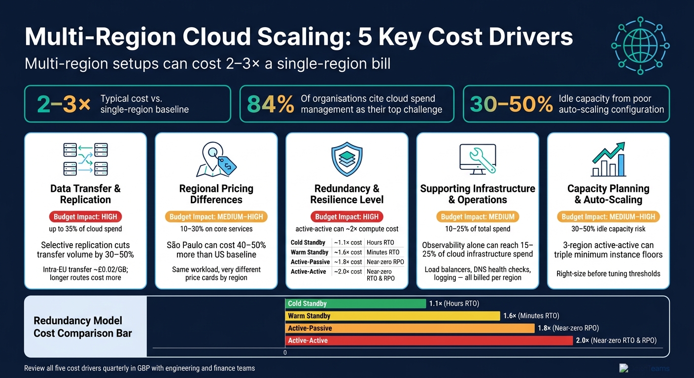 {Multi-Region Cloud Cost Drivers: Key Factors & Budget Impact}
:::
{Multi-Region Cloud Cost Drivers: Key Factors & Budget Impact}
:::
Cloud Cost Optimization for Enterprises: How to Reduce Cloud Costs
Why Multi-Region Costs Rise Faster Than Expected
Multi-region deployments add new layers of cost: duplicated services, replication, failover capacity and region-by-region operations. In practice, the biggest jumps tend to come from three places: duplicated services, traffic moving between regions and the resilience setup itself.
How Duplicated Services Change the Cost Baseline
The moment you add a second region, your starting cost shifts. You now have warm capacity, region-specific managed services and duplicated observability in place before that region handles any user traffic.
That often means compute sitting warm but not running at full load, storage replicated 1:1 for key datasets, and separate charges in each region for logging, alerting and monitoring. Those costs show up whether user demand is high or low. From there, replication settings, region pricing and autoscaling rules decide how fast that new base climbs.
Once traffic, failover and testing are added, the bill usually moves up again.
How Traffic Patterns and Failover Design Affect Spend
Cross-region transfer is often billed per gigabyte, so traffic shape can matter more than server count. A write-heavy workload has to replicate every committed transaction across regions, which can turn a modest setup into a serious monthly transfer charge. DR tests can also push up spend for a short period by lifting secondary-region capacity to match production, causing a spike in that month’s bill. [3][4]
Active-Active, Active-Passive and Cold Standby Explained
The standby model you choose usually sets the upper limit for multi-region spend. [3][4]
| Model | Definition | Cost vs Single-Region |
|---|---|---|
| Active-Active | All regions serve live traffic with near-real-time replication | ~160–200%+ |
| Active-Passive | Primary handles traffic; secondary stays warm and ready | ~130–170% |
| Cold Standby | Minimal secondary footprint; built out only on disaster declaration | ~120–140% |
Active-active fits systems where downtime brings heavy financial or regulatory risk. Active-passive is often the middle option, giving teams a balance between budget and resilience. Cold standby is the lowest-cost setup, but recovery may take hours.
The right choice comes down to a simple trade-off: the cost of downtime versus the cost of resilience. Those trade-offs shape the five cost drivers that follow.
1. Data Transfer and Cross-Region Replication
The more regions you keep in sync, the sooner transfer costs start to beat compute as the main moving part in your bill.
Impact on monthly spend
Every byte that crosses a region boundary is billed on its own. Intra-European inter-region transfer can be around £0.02 per GB, while longer routes cost more.[8][9][2] In most cases, the bill includes transfer charges, replicated storage, and replication requests.[8][9] Once traffic gets high enough, transfer on its own can run into four figures a month.[8][9]
Sensitivity to traffic growth
Replication costs don’t just grow bit by bit. They stack up fast. As write volume goes up, replication traffic goes up with it, and each extra region creates another transfer link. That’s why it makes sense to avoid replicating logs, caches, or non-production data by default.
Selective replication can cut transfer volumes by 30–50% without changing resilience targets.[5][6][12]
Effect on resilience and latency
Synchronous replication keeps data consistent, but it adds wide-area write latency. Asynchronous replication keeps writes faster, but it comes with lag and the risk of data loss during failover.
It’s a trade-off. You’re choosing between tighter consistency and lower write delay.
Optimisation levers
A few changes can make a noticeable dent in these costs:
- Keep read-heavy endpoints and static assets local, and serve them from UK or nearby EU CDN edges.
- Compress replication streams and batch small writes to cut both per-GB charges and request overhead, especially for high-request microservices and log pipelines.[1][7][11]
- Where compliance allows, keep user data local to primary regions and replicate only aggregated or anonymised data for global analytics.
One of the best places to start is simple: build a data-transfer map by region pair and service, then go after the most expensive links first.
After transfer, regional service pricing becomes the next major cost variable.
2. Regional Pricing Differences for Core Services
Once you've mapped transfer costs, the next issue is where each service runs. The same workload can cost very different amounts depending on region. Cloud providers set prices for core services by region based on local costs, demand, and available capacity. So if you're running a multi-region setup, you don't get one neat price card. You get a blended monthly bill pulled from several pricing tables, and that can make forecasting harder than teams often expect.
Impact on monthly spend
Regional price differences can be big. For similar AWS instance mixes, benchmarks suggest that South America (São Paulo) can cost 40–50% more than a US baseline, while Tokyo comes in at roughly 18% higher and Singapore at about 14% higher.[14] Within Europe, the gaps are smaller, but they still matter. Zurich runs about 9% more than Frankfurt, while Stockholm can be around 5% cheaper than Ireland for a similar instance mix.[13]
You can see those differences more clearly when the same workload is priced across regions:
| Service Component | US East (N. Virginia) | London (UK) | Mumbai (India) |
|---|---|---|---|
| AWS Compute (2 vCPU/8 GB) | ~£0.075/hour | ~£0.084/hour | N/A |
| GCP Compute (2 vCPU/8 GB) | ~£0.077/hour | ~£0.077/hour | N/A |
| AWS Storage (10 TB/month) | ~£185.50 | ~£201.70 | ~£201.70 |
| Azure Storage (10 TB/month) | ~£167.75 | N/A | ~£161.30 |
And those gaps don't stay small for long. Once you add managed databases and always-on capacity, the spread gets wider.
Sensitivity to traffic growth
A small hourly difference can look harmless when usage is low. At scale, it's another story. More traffic means more compute hours, more database transactions, and more replication traffic, all charged at that region's rate. Costs can snowball fast, especially in write-heavy systems.
Optimisation levers
The simplest way to think about this is to split the stack by sensitivity. Keep customer-facing and compliance-bound workloads in the regions they need to stay in, usually close to UK or EU users. Then place latency-tolerant parts, like batch jobs and analytics pipelines, in lower-cost regions where the price gap is large enough to matter.
Before you commit, model compute, storage, and database costs by region. Use each provider's pricing calculator to compare the regions on your shortlist. Commitment discounts and right-sizing can also cut the cost of always-on capacity in higher-priced regions, especially where reserved instances or savings plans are available.
3. Redundancy Level and Resilience Strategy
Redundancy is one of the biggest cost drivers in a multi-region setup. The model you pick, whether that’s active-active, active-passive or cold standby, decides how much capacity you’re paying to keep running all the time.
Impact on monthly spend
Active-active can roughly double baseline compute and database spend. Active-passive costs less, but it still adds a fixed monthly bill.
Here’s the simple trade-off: the more ready your standby environment is, the more you pay each month, but the less downtime and data loss you face during a failure.
| Strategy | Typical Cost vs. Single-Region | RTO | RPO | Best For |
|---|---|---|---|---|
| Cold standby | ~1.1× | Hours | Hours | Internal tools, batch workloads |
| Warm standby | ~1.6× | Minutes–1 hour | Minutes | Lower-tier services |
| Active-passive | ~1.8× | Minutes | Near-zero | Important services with some downtime tolerance |
| Active-active | ~2.0× | Near-zero | Near-zero | Customer-facing APIs, payments, identity |
Multi-region databases can cost 80–120% more once replication, duplicate instances and backup storage are included.[15]
Sensitivity to traffic growth
Traffic growth doesn’t hit every setup in the same way. In active-active designs, more traffic pushes up compute, storage, IOPS and replication costs in every live region at the same time. Active-passive is different. Most of that growth stays in the primary region, so the cost curve is usually less steep.
Effect on resilience and latency
Active-active gives you the fastest failover. But there’s a catch: synchronous cross-region writes can add tens of milliseconds of latency when regions are far apart. That delay is part of what you pay for stronger resilience. In plain terms, you’re buying faster recovery, but you may feel it in request speed.
Optimisation levers
A tiered redundancy model usually works best.
- Use active-active for customer-facing APIs, identity and payments.
- Use active-passive or cold standby for internal services and batch workloads.
- Size secondary regions for likely failover demand, not full primary-region parity.
Once redundancy is set, the next cost layer is the extra infrastructure needed to support it.
4. Supporting Infrastructure and Operational Overhead
Once redundancy is in place, the next cost layer comes from the control plane that keeps each region visible and recoverable. In plain terms, every region needs its own load balancers, health checks and monitoring to make failover work.
The problem usually isn’t one big charge. It’s the pile-up of smaller ones. Each region brings its own fixed bill for monitoring and traffic handling, and most of those fees are charged per region, per GB, or per check. That adds up fast. In AWS sample guidance for a two-region deployment, CloudWatch Logs were estimated at £1.21 per month for 1 GB of log data, while an Application Load Balancer came in at £1.54 per month.[17] Route 53 health checks are billed separately at £0.39 per health check per month for AWS endpoints and £0.59 for non-AWS endpoints, with optional features adding another £0.79–£1.58 per month each.[16] Spread those costs across two or three regions and supporting infrastructure can account for 10–25% of total spend in a multi-region setup.
Because CloudWatch is a regional service, you also need separate alarms, dashboards and alerting rules in every region, including the standby.[19] The same pattern shows up in logging tools, metrics pipelines and CI/CD systems. They don’t scale in a neat straight line as you add regions, because each one tends to charge per region, per GB ingested, or per execution.
Sensitivity to traffic growth
Supporting services often grow faster than core compute when traffic climbs. Every user request creates logs, metrics and traces, and in a multi-region setup that can happen in more than one region at once. So a seasonal spike that lifts application compute by 50% can push logging and security event processing up by 80–100%, since each request is tracked more heavily in a resilient multi-region design.
Optimisation levers
The best controls are usually pretty simple:
- Cut log noise at the source by filtering events and tightening retention periods.
- Use one observability stack across regions to avoid duplicate licence costs.
- Automate runbooks so teams spend less time coordinating things by hand.
The standby region should be treated like a live observability target, not a dark corner of the estate. Run canaries, monitor replication lag and track external user experience all the time.[19] Regular failover and failback tests matter too.
Those fixed support costs get harder to absorb once auto-scaling begins reserving spare capacity in every region.
5. Capacity Planning and Auto-Scaling Configuration
When auto-scaling is set badly, each region ends up carrying more capacity than it needs. That extra slack sits there all month, and the bill climbs with it.
Impact on monthly spend
The big issue with multi-region deployments is simple: each region needs its own minimum capacity to meet SLAs, health checks, and failover rules. You can't just think at platform level.
In practice, that can get expensive fast. A 3-region active-active setup can triple minimum instance floors before demand even starts to climb. Databases and caches need regional sizing too, which pushes the baseline up again. So the main cost question isn't just total traffic. It's how much headroom each region has to keep ready before users even show up.
One of the fastest ways to cut this, without touching the core architecture, is to right-size before tuning thresholds. Strip out unused capacity first. Then fine-tune the policies around what's left.[26][24]
Sensitivity to traffic growth
Auto-scaling only keeps costs under control when the metrics match actual demand. CPU on its own is often a late or noisy signal. It's far better to pair it with request rate, queue depth, or latency so the autoscaler can judge when extra capacity is actually needed.[20][18]
It also helps to model growth by region instead of lumping everything together. UK and EU traffic peaks often overlap, while US and APAC peaks tend to land at different times. That matters. A global spike doesn't always hit every region at once, and that's useful when you're planning spend.
A practical way to handle this is to build per-region traffic models that map request volume to instance counts at 10%, 25%, and 50% growth points. That makes it much easier to spot which regions will turn into cost hotspots first, and where scaling thresholds are too loose.
Effect on resilience and latency
Autoscaling helps protect spend in another way: it keeps spare capacity only where failover risk says it's needed.[22][21]
In active-active setups, each region should scale on its own local metrics. If one region gets hit by a traffic spike or drops out, that shouldn't distort scaling decisions elsewhere. The catch is that every region still needs enough headroom to take some failover traffic. A common rule is to size each region for 70–80% of total load, so if one region goes offline, the others can take over without hitting saturation.
Latency trouble usually starts when minimum and maximum scaling limits are set too cautiously. If a region can't add capacity fast enough during a spike, queues build up and tail latency gets worse. That can happen even when other regions still have spare room, because that spare room isn't always easy to shift across in time.
Optimisation levers
A small set of changes usually has the clearest effect on spend:
- Schedule minimum capacity by time of day. If a region has steady quiet periods, it doesn't need the same floor around the clock. Overnight in the UK is a good example.
- Use a baseline-plus-burst model. Put steady-state load on Reserved Instances or Savings Plans, then let auto-scaling add Spot or On-Demand capacity for variable or failover traffic.[23][25][27]
- Add warm pools in regions that see frequent short spikes. That can keep minimum instance counts lower without the hit from cold starts.
- Tune scale-in hard, but safely. Step scaling and graceful connection draining can help remove excess capacity soon after traffic drops.
The same data also shows where outside cost engineering can help most: modelling per-region demand, right-sizing floors, and tuning auto-scaling against billing data. After that, the job becomes pressure-testing those thresholds against billing patterns and failure scenarios.
Where Expert Cost Engineering Can Help
Use expert cost engineering when multi-region spend can't be tied cleanly to a region, service or traffic flow. The five drivers covered in this article - data transfer, regional pricing, redundancy, operational overhead and capacity planning - show where that uncertainty tends to sit. Research suggests 84% of organisations cite managing cloud spend as their top cloud challenge,[30] and only 43% track costs at the unit level,[29] which makes per-region modelling hard to keep up in-house.
When Internal Teams Need Outside Modelling Support
The clearest sign is simple: monthly bills keep climbing, but no one can say which region, service or traffic pattern is behind it. This often shows up during migrations, or when cloud DR runs alongside on-premises DR, and teams can't make a clean cost comparison between retiring one setup and keeping several warm or cold standbys.
Observability is another common pain point. In complex multi-region systems, monitoring costs can reach 15% to 25% of total cloud infrastructure spend,[28] often because logs are forwarded across regions by default, retention periods are set cautiously, and high-cardinality metrics are kept for services that rarely need that much detail.
Hokstad Consulting helps model these costs across replication, scaling and automation decisions.
What to Review in a Multi-Region Cost Audit
Once the spend gap is clear, review each driver in turn. Use the table to match each cost driver to the checks that matter most.
| Cost Driver | Key Audit Review Points |
|---|---|
| Data transfer & replication | Inter-region egress paths, GB/day volumes, replication frequency, compression, unnecessary cross-region forwarding |
| Regional pricing | SKU choices per region, storage tier selection, compute family comparisons, compliance and latency constraints |
| Redundancy & resilience | Secondary-region utilisation vs allocated capacity, RTO/RPO alignment, active-active vs active-passive suitability |
| Supporting infrastructure | Load balancer duplication, logging retention periods, DNS and traffic management services, CI/CD runners per region |
| Capacity planning & auto-scaling | Scaling thresholds vs historical utilisation, minimum instance floors, scheduled scaling rules, UK demand patterns |
The clearest savings usually come from oversized standby regions and duplicated load balancers in low-traffic zones.
Build audit findings into pipelines and governance processes. That includes per-region cost estimates inside infrastructure-as-code templates, logging retention policies tied to actual regulatory needs rather than defaults, and scaling thresholds set against real UK demand patterns instead of cautious, always-on floors. These findings feed directly into the quick cost comparison snapshot that follows.
Quick Cost Comparison Snapshot
Use this side-by-side view to sort the five main cost drivers before you make changes.
| Factor | Cost behaviour | Common triggers | Budget impact | Best mitigation |
|---|---|---|---|---|
| Data transfer & replication | High-growth risk | Unfiltered replication; chatty cross-region calls; no local caching | High - up to 35% of cloud spend [32] | Replicate only critical data; localise services; use CDNs and regional caches |
| Regional pricing differences | Baseline uplift | Region choice without a price check; premium tiers in high-cost regions | Medium to high - 10–30% on core services | Compare per-service prices; place latency-tolerant work in regions that meet latency and compliance needs at lower cost |
| Redundancy & resilience level | Cost multiplier | Active–active by default; critical resilience for non-critical workloads | High - active–active can roughly double compute [31] | Match RTO/RPO to business criticality; use active–passive or cold standby where possible |
| Supporting infrastructure & operations | Steady overhead | Duplicated monitoring/CI/CD; region-specific runbooks | Medium - 5–15% of run costs; observability can reach 25–35% of cloud spend [10] | Share global tooling; centralise logging and monitoring where feasible |
| Capacity planning & auto-scaling | Policy-sensitive | High minimums; excessive buffers; poor thresholds | Medium to high - 30–50% idle capacity | Right-size floors; tune scaling with real demand; test failover load |
Review this table every quarter in GBP with engineering and finance. It gives both teams a simple way to spot what’s driving spend, what’s just background noise, and where action is likely to pay off first.
Conclusion
Multi-region scaling can push spend to around 2–3x a single-region baseline. Why? Because costs stack fast: transfer, regional pricing, redundancy, overhead, and scaling all add up. That’s why line-by-line modelling matters.
Model each cost driver in GBP using current prices for London and any secondary regions. Recheck transfer assumptions on a regular basis, because old estimates go stale fast. It also helps to track each line item on its own and review it every quarter with engineering and finance.
From there, the key question isn’t simply whether to go multi-region. It’s whether the resilience gain is worth the extra spend. Choose multi-region only when your RTO/RPO targets clearly justify the added cost.
If your team doesn’t have the time or in-house experience to model this with confidence, Hokstad Consulting helps UK organisations map multi-region costs and turn infrastructure choices into clear GBP forecasts. That makes it easier to decide which regions should stay, scale, or go.
Run each region only when it earns its place on resilience, performance, and total cost.
FAQs
When is multi-region worth the extra cost?
Multi-region is worth the extra cost when the business value of performance, resilience, and regulatory compliance is higher than the added complexity and ongoing spend.
It tends to make sense for mission-critical applications that need high availability, disaster recovery, data residency, or lower latency for users spread across the globe. Before you scale, compare the business cost of downtime with the price of cross-region data transfer, replication, and load balancing.
Which workloads should not be replicated across regions?
To cut cloud spend, don’t replicate workloads that don’t care about low latency. Batch processing and data warehousing are good examples. They can often run in lower-cost regions farther away, because distance doesn’t affect how they perform.
The same goes for internal systems and non-critical backups where speed isn’t a priority. There’s no point mirroring them in premium locations if the business gets little in return. Look at each workload in terms of business value, and check whether the extra cost of data transfer and infrastructure synchronisation is worth paying.
How often should we review multi-region cost assumptions?
Review multi-region cost assumptions on a regular basis so they still match shifting business goals and cloud pricing. For many teams, a check every three or six months is enough to spot problems like misconfigured scaling or orphaned resources before they quietly add to the bill.
Recovery-focused plans and drills should get a quarterly review too. Regular monitoring, with input from both technical and finance teams, helps keep spend under control as regional setups become more complex.