Grafana Tempo: Cost-Effective Kubernetes Tracing

Grafana Tempo simplifies distributed tracing in Kubernetes by tracking requests across services without relying on expensive databases. By using object storage like Amazon S3, Tempo reduces costs and complexity while handling large trace volumes. It integrates with Prometheus and Loki, offering seamless observability for debugging and performance monitoring. Tempo’s modular architecture supports both small-scale and high-volume workloads, making it a practical choice for organisations managing complex microservices.

Key Highlights:

• No-index architecture: Stores trace data in object storage, cutting costs significantly.
• Kubernetes-friendly: Components can scale independently for high-traffic environments.
• Unified observability: Links metrics, logs, and traces in a single interface.
• Cost-efficient scaling: Enables 100% trace sampling without increasing expenses.

For UK deployments, Tempo supports regional object storage to meet data residency requirements and reduce latency. With Helm charts, it’s easy to deploy and configure Tempo in Kubernetes, ensuring efficient trace retention and performance monitoring.

Tempo + Alloy + Grafana: Kubernetes Distributed Tracing

Grafana Tempo Architecture and Scalability

::: @figure 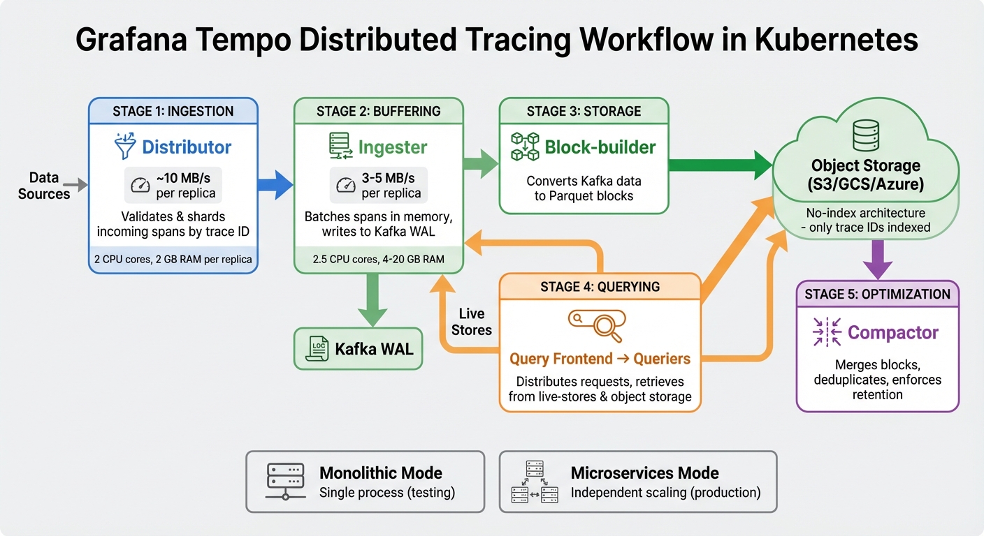{Grafana Tempo Architecture: Components and Data Flow in Kubernetes} :::

Main Components: Ingestion, Storage, and Query Layers

Grafana Tempo is built around a modular architecture designed to handle distributed trace processing efficiently. Each key component plays a distinct role and can be scaled separately to meet production demands.

The Distributor handles incoming spans from applications, validating and sharding data based on trace IDs. This ensures load is evenly distributed across the system. A single distributor replica can manage approximately 10 MB/s of traffic [6].

The Ingester temporarily stores spans in memory, batching them before writing to a Kafka-compatible write-ahead log. This setup separates the write and read paths, so high ingestion rates don't interfere with query performance. Typically, each ingester replica processes 3–5 MB/s of data [6].

The Block-builder takes data from Kafka and converts it into compressed blocks using the Apache Parquet format. These blocks are stored in object storage, a highly efficient and compressed format optimised for querying [2].

For querying, the Query Frontend distributes incoming requests across multiple Queriers, which retrieve trace data from both live-stores and historical object storage. The Compactor plays a crucial role in merging smaller blocks, deduplicating data, and enforcing retention policies [2].

Grafana Tempo supports two operational modes:

• Monolithic mode: All components run within a single process, ideal for testing environments.
• Microservices mode: Each component operates independently, allowing for separate scaling. This mode is essential for Kubernetes deployments handling large trace volumes.

This flexible setup ensures Tempo can handle high trace volumes while keeping costs manageable.

Reducing Costs with Object Storage

One of Tempo's standout features is its ability to minimise costs through the use of object storage. Unlike traditional tracing systems like Jaeger or Zipkin, which rely on complex databases such as Elasticsearch or Cassandra to index traces, Tempo uses a no-index architecture. It only indexes trace IDs, significantly reducing storage and computational overhead [1][3].

Backend Engineer Akash Sahani highlights this advantage:

Tempo only requires object storage to operate and supports common protocols like Jaeger, Zipkin, and OpenTelemetry [3].

By utilising cost-efficient object storage solutions like Amazon S3, Google Cloud Storage, or Azure Blob Storage, Tempo enables massive scalability at a fraction of the cost associated with index-heavy databases [2][7]. For instance, storing 1 TB of trace data in object storage through Tempo is substantially cheaper than using traditional database systems [8].

In March 2023, an organisation reported a 50% reduction in operational costs after switching from a database-backed tracing system to Tempo's object storage model. This shift allowed them to scale their tracing capabilities without increasing expenses [Grafana Tempo documentation, 2023].

This cost-efficient design also enables organisations to sample 100% of their traces, eliminating the need for aggressive sampling strategies often used to control costs. This represents a transformative approach to distributed tracing [1][3].

Deploying Grafana Tempo on Kubernetes

Installing Tempo with Helm Charts

To deploy Grafana Tempo on Kubernetes (v1.29+ with Helm 3+), you’ll need a node with at least 6 cores and 16 GB of RAM, along with persistent storage configured [9]. Start by creating a dedicated namespace, such as tempo, to keep Tempo resources organised [9]. Then, add the Grafana community Helm repository using:

helm repo add grafana-community https://grafana-community.github.io/helm-charts

Update the repository with:

helm repo update

The tempo-distributed Helm chart sets up multiple microservices, including the distributor (for processing spans), the ingester (for in-memory buffering), the querier (for retrieving traces), the query-frontend (for request distribution), and the compactor (for managing storage). Each service can scale independently, making it suitable for production environments [9][10].

Configuration is handled through a custom.yaml file where you specify the storage backend, trace receiver protocols (like OTLP, Jaeger, or Zipkin), and resource allocations. To optimise resource use and reduce potential vulnerabilities, only enable the protocols your applications actually require [9][10]. For UK-based deployments, consider creating S3 buckets in local regions, such as eu-west-2 (London), to meet data residency requirements and reduce latency [10].

Avoid using the built-in MinIO for production, as it has a 5 GiB storage limit [9]. Instead, set up a production-grade object storage solution right from the start. Once Tempo is deployed, you’ll need to configure your object storage backend for effective trace retention.

Setting Up Object Storage for Trace Retention

After deployment, configure object storage to manage Tempo’s trace retention efficiently. This involves defining storage settings in your custom.yaml file, typically using services like Amazon S3, Azure Blob Storage, or Google Cloud Storage. Specify the bucket name and region to ensure proper configuration [10].

For AWS, it’s better to use IAM Roles for Service Accounts (IRSA) instead of embedding access keys. Annotate the service account in your Helm setup to securely grant Tempo pods access to your S3 bucket [10]. For deployments in the UK, set the endpoint to s3.eu-west-2.amazonaws.com to minimise data egress costs and latency [10].

Trace retention is managed by the compactor service, which determines how long trace blocks are stored before being deleted. Adjust the block_retention parameter based on your debugging and service-level needs - for instance, 72h for three days or 168h for a week [11][10].

Nawaz Dhandala, a Software Engineer, highlights the role of infrastructure as code in this process:

Deploying Tempo via Flux CD means your ingestion configuration, retention settings, and S3 block storage parameters are version-controlled [11].

Additionally, configure S3 lifecycle rules to automatically remove objects after the retention period, with a small buffer to account for delays. This prevents unused objects from building up and driving up storage costs. Using a dedicated bucket for Tempo traces, separate from logs or metrics, can also simplify both cost tracking and lifecycle management [11].

Optimising Grafana Tempo for Cost and Performance

Configuring Retention Policies and Metrics Generator

To cut down on object storage costs, adjust the compactor's block_retention setting. For example, use 168h for standard workloads, 336h for critical services, or tiered values for multi-tenant setups. In multi-tenant environments, you can apply per-tenant overrides, such as assigning 48h for trial accounts while reserving 720h for premium customers [13].

The Metrics-generator can summarise trace data into Prometheus metrics, but it's crucial to limit label dimensions - for instance, using only service.name and http.status_code. This keeps series cardinality manageable [12]. Keep an eye on tempodb_compaction_outstanding_blocks and set compacted_block_retention to 1h to ensure small blocks are merged efficiently, avoiding query performance issues [13].

Additionally, configure max_attribute_bytes to a maximum of 2048 bytes to truncate overly large span attributes [5]. Andreas Gerstmayr, a Software Engineer at Red Hat, highlights the simplicity of Tempo's storage requirements:

Tempo requires only object storage for storing traces, which is easy to set up in both cloud environments and on-premises. [4]

These configurations are essential for keeping trace management cost-effective and efficient, especially in Kubernetes environments.

Monitoring Tempo Pods in Kubernetes

Once retention and performance settings are optimised, it's critical to monitor Tempo pods to ensure they operate efficiently and detect any issues early. Each Tempo component has specific resource needs. For example:

• Distributors typically need one replica per 10 MB/s of incoming traffic, with each replica requiring around 2 CPU cores and 2 GB of RAM [6].
• Ingesters and Compactors generally need one replica per 3–5 MB/s of traffic. Ingesters, in particular, require about 2.5 CPU cores and between 4 and 20 GB of RAM, depending on the trace composition [6].

To automate monitoring, deploy ServiceMonitor objects, enabling Prometheus to scrape metrics from all Tempo pods [10]. Set up alerts for key issues like distributor push errors exceeding 1%, ingester flush failures, and query latencies above 30 seconds at the 99th percentile. Additionally, enable cost_attribution via /usage_metrics to track service-specific ingested bytes [14]. This data can pinpoint which services or teams are driving storage costs, making it easier to adjust retention policies and allocate resources wisely.

Scaling Grafana Tempo for High-Volume Workloads

Managing High Trace Volumes

Scaling Grafana Tempo to handle millions of spans per second requires careful planning and the right architecture. Instead of relying on a single monolithic instance, Tempo operates in a distributed mode. Its components - Distributors, Ingesters, Queriers, and Compactors - are deployed as independent services. This allows horizontal scaling of specific components to accommodate increasing trace volumes without overprovisioning.

One of Tempo's standout features is its ability to write traces directly to object storage (like S3, GCS, or Azure Blob). By bypassing the traditional indexing layer, Tempo avoids the scaling limitations often seen with index databases. As DevOps professional Keval Bhogayata puts it:

Tempo takes a fundamentally different approach by writing traces directly to object storage... skipping the indexing layer entirely [8].

This design not only simplifies scaling but also makes storing large amounts of trace data - such as 1 TB - far more cost-efficient compared to indexed systems.

For environments with extremely high traffic, head-based sampling via the OpenTelemetry Collector's probabilistic sampler is a practical solution. This method ensures that all error traces are captured while sampling only a fraction of successful requests, keeping both storage and processing costs under control. Additionally, Tempo's built-in multi-tenancy allows teams within the same cluster to isolate their data and set per-tenant ingestion and retention limits, streamlining operations and maintaining cost efficiency [8].

Combining Tempo with Prometheus and Loki

Tempo's real power shines when integrated with Prometheus and Loki, forming a cohesive observability stack. This combination enables workflows that connect metrics, traces, and logs seamlessly. For example, exemplars in Prometheus can link directly to Tempo Trace IDs, allowing you to jump from a metric spike to the exact trace causing the issue. From there, it's easy to correlate the trace with relevant logs.

Tempo also supports automation through its Metrics Generator, which creates Prometheus metrics directly from trace data. These metrics include service graphs and span metrics like request rates and latencies. This automation reduces the need for manual instrumentation and eliminates the inefficiencies of ad-hoc trace searches, ensuring that Trace IDs remain consistent across metrics, traces, and logs. This consistency aligns perfectly with Tempo's focus on providing scalable and low-cost trace storage [8].

In Kubernetes production environments, high availability and scalability are essential. Use Horizontal Pod Autoscalers set to maintain 70% CPU utilisation for components like Distributors, Ingesters, and Queriers to handle traffic spikes effectively. Adding Memcached to cache trace data can further improve query speeds by reducing the number of GET requests to object storage.

For more detailed advice on optimising Grafana Tempo deployments in Kubernetes, Hokstad Consulting offers expert guidance tailored to cost-effective solutions.

Conclusion

Grafana Tempo streamlines distributed tracing within Kubernetes environments by writing traces directly to object storage, completely bypassing the need for an indexing layer. This approach not only simplifies operations but also significantly lowers costs. For example, storing 1 TB of trace data is far more affordable compared to traditional indexed systems like Elasticsearch [8].

For UK businesses aiming to optimise their cloud infrastructure, Tempo offers independently scalable components - Distributor, Ingester, Querier, and Compactor - that allow Kubernetes clusters to process millions of spans per second. Additionally, the use of regional S3-compatible storage ensures compliance with data residency requirements while maintaining deployment flexibility. This scalability complements the unified observability framework that Tempo integrates with Prometheus and Loki.

Tempo’s design also enables seamless integration with Prometheus and Loki using exemplars, creating a unified observability workflow that helps reduce Mean Time to Resolution. As Roman Vogman from Houzz highlights:

Having it all in one tool like Grafana Cloud Traces simplifies the process [15].

With Grafana Cloud offering up to 50 GB of traces per month for free and self-hosted deployments incurring only object storage costs, Tempo provides a cost-effective and scalable solution. It aligns perfectly with cloud-native growth strategies, making it an appealing choice for businesses. For those looking to optimise their DevOps and cloud infrastructure, Hokstad Consulting offers expertise in reducing operational costs and improving system observability.

FAQs