
If I had to boil this down to one point, it’s this: multi-cloud mesh observability works when I standardise labels, keep collection close to each cluster, and only centralise the data I need.
Running services across AWS, Azure and GCP is common enough. But once traffic moves between clusters and clouds, metrics, logs and traces split across tools, regions and teams. That creates blind spots, higher spend, and slower incident work. The article’s main answer is simple: use one telemetry model, local collectors in every cluster, and a hybrid backend design that balances cost, query needs and data location rules.
Here’s the short version:
-
Metrics tell me what is failing now:
- request rate
- p95/p99 latency
- error rate
- saturation
-
Logs tell me what happened in detail:
- proxy access logs
- gateway logs
- control-plane logs
- correlation IDs for incident work
-
Traces tell me where a request went:
- cross-cluster path
- retries and timeouts
- failover between clouds
- span-level timing
-
The setup that keeps order:
- sidecars and gateways emit telemetry
- one OpenTelemetry Collector per cluster
- Prometheus for local metrics
- Loki for logs
- Tempo, Jaeger or Zipkin for traces
- central views for SLOs and cross-cloud incidents
-
The big risks:
- broken or mixed labels like
prodvsproduction - high-cardinality labels driving storage bills
- egress costs from shipping raw telemetry across clouds
- weak trace propagation between app code and proxies
- broken or mixed labels like
-
The cost picture matters:
- observability can take 15%–25% of cloud spend
- large estates can pass £50,000 per month
- moving custom metrics from 1-minute to 5-minute resolution can cut cost by about 5×
- governance can reduce spend by 20%–40%
-
The design choice that matters most:
- centralised backend: simpler global querying, but more egress cost
- regional backends: lower transfer cost and better data location control, but harder cross-region investigation
- hybrid: local raw data, central aggregates and sampled data
A quick comparison of the three mesh options covered:
| Mesh | Best fit | Telemetry control | Complexity |
|---|---|---|---|
| Istio | Fine-grained control across clusters | High | High |
| Linkerd | Lower-overhead golden signals | Medium | Low |
| Consul | Hybrid and multi-datacentre estates | High | Medium |
I’d read the rest of the article as a guide to one job: how to get one usable view of a multi-cloud service mesh without letting cost, drift and tooling sprawl get out of hand.
::: @figure 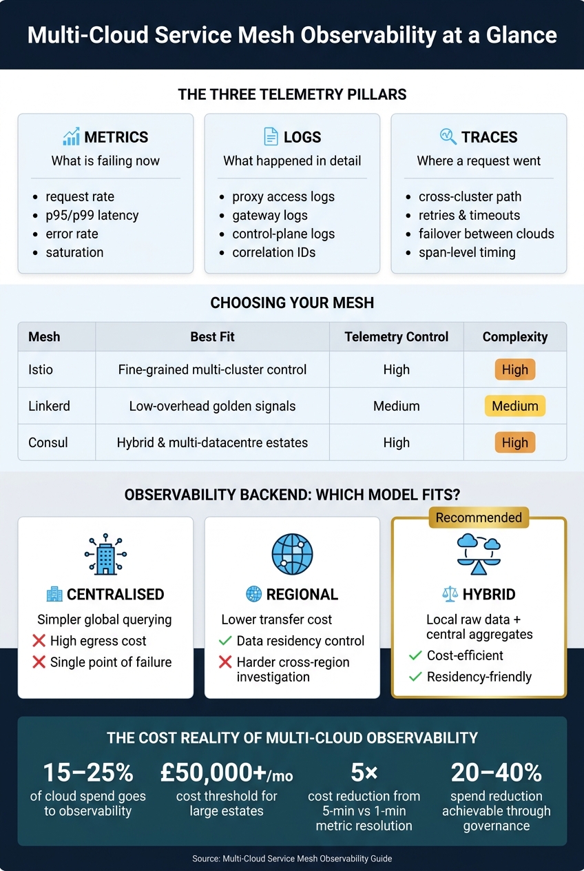 {Multi-Cloud Service Mesh Observability: Architecture & Cost Comparison}
:::
{Multi-Cloud Service Mesh Observability: Architecture & Cost Comparison}
:::
Multi-Cluster Observability with Service Mesh - That Is a Lot of Moving Parts!? - Ryota Sawada
Telemetry architecture for multi-cloud meshes
The three telemetry pillars only matter if data moves through one steady collection path across every cluster. In a single cluster, that’s pretty easy. In a multi-cloud mesh, it isn’t. You need to collect, normalise and query telemetry from one place.
So the main issue isn’t what to collect. It’s where each signal enters the pipeline and how you standardise it before storing it. In practice, that pipeline has five layers: sidecar and dataplane proxies, mesh control planes, ingress and egress gateways, per-cluster collectors, and central storage and visualisation.
How dataplane and control-plane telemetry flows across clouds
Sidecar proxies sit directly on the request path, so they see every call as it happens. They emit per-request metrics, logs and traces. Envoy scrapes metrics from /stats/prometheus on a dedicated port such as 15020, sends structured access logs to a log agent, and exports trace spans through OTLP to an OpenTelemetry Collector.[3][5]
Control planes add a different set of signals. They show you what’s happening with config and security, including reconciliation latency, xDS push errors, certificate issuance and related logs.
Ingress and egress gateways are useful choke points for cross-cloud traffic. If you label gateway metrics by source cluster, destination cluster and cloud provider, you can see inter-cloud traffic volume, latency and error rates far more clearly. Gateway trace spans also mark the boundary between clusters, which lets a tracing UI rebuild the path a request takes as it moves between clouds.
A common setup is to run an OpenTelemetry Collector in each cluster. That gives you a place to normalise labels, sample traces and forward telemetry to a central backend. For metrics, use Prometheus remote write to Thanos, Cortex or Mimir. Federation is better kept for limited read-only aggregation. For traces, collectors can apply tail-based sampling so only high-value traces are forwarded, which cuts cross-cloud bandwidth use and storage spend.
Observability patterns in Istio, Linkerd and Consul Service Mesh
Each mesh exposes telemetry in its own way, so your collection approach needs to match the control plane you already use. The design changes because defaults, labels and sampling controls are different in each product.
Istio gives you the deepest telemetry control of the three. Its Telemetry API manages metric sets, access log formats and trace sampling at workload, namespace or mesh level. Istio’s production tracing example uses 10% sampling as a starting point.[4] In multi-cluster setups, Istio tags spans with source_cluster and destination_cluster, which means you can rebuild cross-cloud call graphs. The downside is plain enough: Istio is harder to run well, and keeping telemetry steady across clusters takes care and planning.
Linkerd goes the other way. Its opinionated defaults and lightweight Rust proxy make it much simpler to run, and its built-in golden-metrics dashboards give fast SLO visibility out of the box. It also supports multi-cluster traffic through service mirroring and gateways, and its metrics can show which endpoints are meshed and which are not. The weak spot is control depth: you get less per-hop tracing and less log-format control, so deep cross-cloud path analysis can be harder.
Consul Service Mesh fits hybrid and multi-datacentre setups well. Its control plane exposes metrics for service registration, health checks and WAN federation behaviour. Those signals matter when part of a stack runs in a UK on-premises data centre and the rest runs in public cloud. Consul’s service tags and namespaces can encode location and regulatory domain, and that context can flow into metrics and traces across mixed infrastructure.
| Mesh | Telemetry types | Multi-cluster labelling | Tracing flexibility | Operational complexity |
|---|---|---|---|---|
| Istio (Envoy) | Metrics, access logs, traces |
source_cluster / destination_cluster tags |
High - OTLP, configurable sampling | High |
| Linkerd | Metrics, tap/live inspection, traces via integrations | Meshed vs non-meshed endpoint metrics | Moderate - fewer native controls | Low |
| Consul (Envoy) | Metrics, access logs, traces | Service tags, namespaces, DC labels | High - Envoy tracing integrations | Moderate |
Use Istio when you want fine-grained telemetry control, Linkerd when you want low-overhead SLO visibility, and Consul when hybrid setups and federation matter most.
Implementing metrics, logs and traces at scale
This section turns the architecture into pipelines you can deploy. The base setup has three of them: metrics, logs and traces. Each choice affects visibility, latency and cost across cloud boundaries. From here, the job is to pick collection, storage and sampling patterns that match your service mesh and your budget.
Metrics collection with Prometheus, remote-write and long-term storage
Start with metrics in each cluster. Then centralise only the data you need for cross-cloud SLOs.
Run one Prometheus instance per cluster, scoped to mesh parts. Scrape sidecars, gateways and control-plane pods with ServiceMonitor and PodMonitor. Use 15- to 30-second scrape intervals for critical services, and slower intervals for everything else.[15][13]
Use the same cluster, region, cloud_provider and mesh labels from day one.[14][15]
For long-term storage and global queries, use Prometheus remote-write to Thanos or Cortex/Mimir. Thanos stores TSDB blocks in object storage such as S3-compatible storage, GCS or Azure Blob. It also down-samples older data into 5-minute and 1-hour resolution tiers, which helps keep long-range queries responsive and storage spend lower.[7][9][10] To cut cross-cloud egress, send remote-write traffic to a receiver in the same cloud region where you can. Then use federated queries for global aggregation instead of shipping raw time series between providers all the time.
Keep alert rules inside each cluster's Prometheus so incident response stays fast and low-latency. A central Alertmanager can then aggregate and deduplicate alerts across clusters to give you one global view.[15][16] If you're working in a UK organisation, tie SLO breaches to £ impact. For example, if a checkout service brings in £10,000 per hour and success drops to 50%, annotate the alert with a £5,000-per-hour exposure.[15][16]
Centralised logging for sidecars, gateways and control planes
Logs need their own design. Volume, retention and query patterns are not the same as metrics or traces.
The rule is simple: keep collection local, centralise only what gets queried often, and keep high-volume data for the shortest time you can justify.
Run Promtail or Fluent Bit as a DaemonSet in each cluster. Use namespace or label selectors to route dataplane logs, such as HTTP access logs, gRPC summaries and TLS handshake records, and control-plane logs, such as configuration changes, reconciliation loops and leader-election events, into separate Loki streams. Ship logs over TLS to shared Loki, labelled with cluster, cloud, region and environment.[6] Avoid high-cardinality values like user IDs or request IDs as Loki labels. At scale, index bloat gets expensive fast.
Keep production access logs for 3 to 7 days. Keep control-plane or security logs for 30 to 90 days. Retention by log type and environment keeps storage under control without giving up audit needs.
| Logging approach | Multi-cluster support | Query depth | Retention control | Primary cost driver |
|---|---|---|---|---|
| Centralised (single Loki) | Good - single ingestion point | Deep cross-cluster correlation | Global policies, less granular | Cross-region egress, central storage |
| Regionally distributed Loki | Excellent - local ingestion | Deep within region only | Per-region policies | Operational overhead, cross-region query gaps |
| Hybrid tiered (local + central archive) | Good - local for speed, central for history | Deep locally, summarised centrally | Fine-grained by tier | Replication cost, pipeline complexity |
Distributed tracing with OpenTelemetry and mesh-generated spans
Tracing is the hardest stream to scale, so sampling comes first.
Use the same rule as before: keep collection local, centralise only what gets queried often, and keep high-volume data for as little time as possible.
Deploy one OpenTelemetry Collector per cluster to receive spans from mesh proxies and application SDKs over OTLP. Mesh proxies create spans for every sidecar hop, including retries, circuit-breaking events and TLS handshakes. Application-level spans show business steps such as order validation or payment processing. Put both together and you get an end-to-end view from the user's entry point, across network boundaries, through internal functions, and across clouds.[11][12]
Trace context moves through the W3C traceparent header, which Envoy and Linkerd proxies forward on their own. Application code also needs to pass traceparent. If it doesn't, mesh spans and app spans split into separate traces. Add cluster, cloud, region and service attributes during collector enrichment so the backend can rebuild cross-cloud call chains without confusion.
Sampling matters even more in multi-cloud than in a single cluster, because full-fidelity tracing across cloud boundaries can drive up egress. Head-based sampling at the proxy cuts volume at the source. Tail-based sampling in the collector lets you keep traces that cross error or latency thresholds, even if the first sampling choice would have dropped them. Tempo often keeps production, staging and development traces for 14 days, which is a useful short-term retention benchmark.[8]
| Backend | Storage model | Retention | Query capabilities | Multi-cloud deployment complexity |
|---|---|---|---|---|
| Jaeger | Elasticsearch or Cassandra | Moderate - index costs rise at scale | Rich: service, operation, tag and time-range search | Medium-high; needs tuned storage per region |
| Grafana Tempo | Object storage (S3-compatible) | Long-term at low cost; no field indexing | Trace ID lookup; best combined with Loki and Prometheus exemplars | Low-medium; object storage is available in all major clouds |
| Zipkin | In-memory or Elasticsearch | Short-term by default | Basic trace and dependency graph search | Low; lightweight but limited at high scale |
Tempo's object-storage model makes it a good fit for multi-cloud setups where trace volume is high and long retention matters. Jaeger is still a solid choice when rich field-level querying matters and the team already runs Elasticsearch. Zipkin fits lower-scale setups or teams that want a simple place to start.
Need help optimizing your cloud costs?
Get expert advice on how to reduce your cloud expenses without sacrificing performance.
Building a unified, cost-aware observability platform
Centralised versus regionally distributed observability backends
Once your collection pipelines are in place, the next call is simple in theory and messy in practice: where does telemetry live, and where do you query it from? That choice shapes cost, resilience and compliance.
A centralised backend sends everything to one place. It’s easier to run, and it makes cross-cloud correlation much simpler because teams can query data in one backend. But there’s a catch. Moving raw telemetry from many clouds and regions into one location can create high cross-cloud egress charges, and the central backend can turn into a single point of failure for your visibility layer.
Regionally distributed backends take the opposite route. Raw, high-volume telemetry stays close to where it was generated, with each cloud or region running its own observability stack. Then the central layer is used for global SLOs and cross-cloud incident correlation, rather than for storing all raw telemetry.
| Factor | Centralised backend | Regionally distributed backends |
|---|---|---|
| Latency | Higher - data travels to central hub | Lower - local ingestion and queries |
| Resilience | Single point of failure for visibility | Regional failure affects only that region |
| Ops overhead | One backend to manage | Multiple stacks; risk of configuration drift |
| Data residency | Harder - requires careful routing | Easier - data stays in-region by default |
| Egress cost | High - all raw data crosses providers | Low - only aggregates or samples forwarded |
For most UK organisations, the practical option is a hybrid model: regional backends for raw telemetry, plus a central aggregation layer for SLO dashboards and cross-cloud incident correlation. Multi-cloud observability often makes up 15–25% of total cloud infrastructure spend[1], so this isn’t just an architecture choice. It has a direct effect on your monthly bill in £.
That model only holds up if retention, sampling and access rules are applied the same way everywhere.
Cost control, tenancy and access governance
Cost control starts with labels and retention, then moves into a harder question: who gets to see what?
Telemetry volume is usually the main cost driver, and in a service mesh it climbs fast. Every sidecar hop can generate spans, access logs and metrics. One of the strongest levers here is metric downsampling. Moving custom metrics from 1-minute to 5-minute resolution can deliver about a 5× cost reduction[18] for those series. Pair that with cardinality control - for example, avoiding high-cardinality labels such as request IDs or user IDs on mesh metrics - and storage costs can drop sharply. Organisations that put telemetry governance in place have reported cuts in observability spend of 20–40%[17] without a meaningful loss in operational capability.
Retention policy matters just as much. Production access logs often need only 7–14 days of full-fidelity retention for incident response. Control-plane and security logs usually need longer. Compliance-only archives can move into low-cost object storage with infrequent access. Applying those tiers across clouds, and enforcing them through Fluent Bit or OpenTelemetry Collector configuration, helps stop storage costs from quietly piling up until the next quarterly cloud bill lands.
In multi-team setups, three governance actions matter most:
- Standardise labels such as
tenant,team,business_unit,environment,cloud_providerandmesh_clusteracross every sidecar-generated telemetry stream. That makes chargeback and showback possible, so the cost of cross-cloud mesh traffic can be tied back to the teams creating it. - Enforce RBAC across all observability backends. Raw logs and full traces may include transaction metadata or customer identifiers, so access should be limited to authorised roles.
- Enable audit logging on the observability tools themselves, so you can track who queried what and when.
In regulated UK sectors - financial services, healthcare and the public sector - these controls aren’t optional. A central identity provider with SSO using OIDC or SAML helps keep access policies aligned across AWS, Azure, GCP and on-premises stacks.
How Hokstad Consulting can help
These choices are hard to standardise when different teams, clouds and compliance rules all pull in different directions. Hokstad Consulting works with platform teams on cloud cost engineering and DevOps transformation, including cost audits, monitoring architecture and infrastructure automation, to reduce cloud spend by 30–50%. That work targets excess egress spend, compliance gaps and alert fatigue, which tend to bite hardest as observability costs climb in hybrid and multi-cloud estates.
Advanced practices and conclusion
eBPF, zero-code instrumentation and AI-assisted incident detection
Once your core telemetry pipelines are steady, the next move is to cover the blind spots that sidecars and app agents miss. eBPF (extended Berkeley Packet Filter) hooks into the Linux kernel to watch network traffic, TCP retransmissions, syscall patterns and packet drops across every pod and node. That includes DNS, kubelet and CNI activity. It works with mesh telemetry, not instead of it.
Here’s why that matters. If a p99 latency alert goes off, eBPF can help show whether the issue comes from a noisy neighbour, disk I/O saturation, or a packet drop on a specific interface. That can cut root-cause analysis time by a lot. With local collectors and selective sampling, eBPF gives you more depth without swamping the backend.
For services that can’t be instrumented by hand, OpenTelemetry's eBPF Instrumentation (OBI) can capture trace spans and RED metrics for Linux HTTP/S and gRPC traffic without code changes.[19] That helps extend coverage across estates where full app instrumentation just isn’t practical. Pair OBI with a shared OpenTelemetry Collector DaemonSet set up the same way across clouds, and you can get broad coverage without touching app code.
Add AI-assisted detection on top of that telemetry - such as anomaly detection and log or trace summarisation - and teams spend less time digging through dashboards by hand. A multi-cloud DevOps observability study found that organisations using unified observability architectures saw a 63% average reduction in mean time to incident diagnosis and 71% faster cross-provider latency diagnosis than with their previous approach.[2] In plain terms, triage gets faster because AI can connect signals across regions and clouds more quickly than manual dashboard review.
The key difference comes down to what the tool can see. Some tools learn only from the mesh. Others correlate mesh data with kernel and app signals too. That changes how fast they spot issues and how much noise they produce.
| Aspect | Traditional dashboards & alerts | AI-assisted observability |
|---|---|---|
| Detection speed | Static thresholds; slow across clusters. | Learns service, region and mesh baselines; flags anomalies earlier. |
| Noise reduction | Alert storms during major incidents; hard to maintain quiet-but-safe thresholds. | Correlates alerts, suppresses duplicates and adapts thresholds over time. |
| Skills required | Strong SRE/DevOps expertise to design dashboards and interpret signals manually. | Skills to configure AI pipelines; less manual threshold tuning; SRE oversight still needed. |
| Effect on MTTR | Depends on people who know mesh topology and historical incidents. | AI surfaces likely root causes and summarises traces and logs, speeding triage. |
One governance point needs to be said plainly: before sending logs and traces into any AI engine, scrub personal data and secrets, and apply RBAC by tenant, region and environment. Human review should still stay in place for high-severity or unclear incidents.
Taken together, these techniques push visibility beyond collection and into diagnosis.
Conclusion: core design choices for reliable multi-cloud visibility
A small set of decisions shapes whether multi-cloud mesh observability works day to day. Define a standard telemetry model first. Add consistent attributes - service_name, cloud_provider, region, cluster_id, mesh_name, tenant, environment - to every metric, log and trace. That gives cross-cloud queries and AI-assisted correlation a solid base. Without it, every later step becomes harder to defend.
Instrument metrics, logs and traces together. Every user-facing critical path needs latency and error metrics, access logs with correlation IDs, and end-to-end traces that carry context across services and regions. Treat them as separate tracks, and you create the very gaps that make cross-cloud incidents drag on.
Choose the topology that fits your retention, residency and egress limits. A centralised backend makes global SLOs and AI-assisted analysis simpler, but it can increase egress costs. A federated model keeps raw data local and helps meet data residency rules, but cross-region investigations become more awkward.
Finally, tie retention and sampling to business value. Use tail-based sampling to keep the traces that help most with diagnosis. Apply tiered retention: shorter windows for high-resolution data, longer periods for aggregates and SLO trend analysis. Label telemetry by tenant and region so chargeback in £ is possible. That keeps spend under control while still supporting incident diagnosis.
FAQs
Which telemetry should I centralise first?
Start with metrics to get a clear view of traffic flow, performance and service health across your multi-cloud mesh.
At the same time, collect request traces so you can see how services interact across clusters and cloud providers. Use open standards such as OpenTelemetry to standardise logs, metrics and traces as you bring them into one shared backend.
How do I reduce observability costs in a multi-cloud mesh?
Cut observability spend by shifting away from reactive monitoring and towards a leaner plan. A good place to start is with vendor-neutral standards such as OpenTelemetry. That gives you more freedom, helps cut tool sprawl, and makes it easier to bring logs, metrics and traces into one platform instead of paying for the same view in several places.
Storage is another area where costs creep up. Review your retention policies so you’re not paying to keep old data that no one uses. A lot of teams hang on to historical records for too long simply because no one has gone back to check what still matters.
It also pays to tune your observability agents properly. If they use too much CPU and memory, you’re spending more than you need to just to watch your systems. On top of that, use automation and Infrastructure as Code to keep tagging consistent and to spot underused services or duplicate data streams before they turn into a bigger bill.
What most often breaks cross-cloud tracing?
Most often, cross-cloud tracing falls apart because tools and monitoring systems don't work cleanly across providers. That creates data silos, which makes end-to-end correlation hard or, in some cases, impossible.
Other common causes include:
- inconsistent cluster naming
- misconfigured monitoring endpoints
- lost trace context across service boundaries
- in service meshes, failing to manually set up a shared root of trust across clusters