
Multi-cluster CI/CD can lower costs by 24–33% in many cases, but it can also add a lot of waste if jobs land in the wrong place. I’d look at four things first: compute use, spot capacity, cross-cluster traffic, and £ per pipeline run.
Here’s the short answer:
- Lower compute spend usually comes from tighter packing, better resource requests, and using spot nodes for restart-safe jobs.
- Higher costs often come from idle capacity spread across clusters and egress charges when artefacts, images, or test data cross regions or clouds.
- Shared or hybrid cluster layouts often cost less than fully separate setups, but they need tighter controls.
- The metric I’d track is £ per workflow, not just total cluster spend.
A few numbers stand out:
- Smart scheduling has been linked to 24–33% lower execution cost.
- Spot or pre-emptible nodes can cut compute prices by 60–90% for the right jobs.
- Dynamic placement across clusters tends to save 5–20%.
- One case saw US$1.3 million in egress fees from poor traffic control.
- Many clusters start at only 20–30% use before tuning.
If I were putting this into practice, I’d keep the plan simple:
- Send build and test jobs to the cheapest safe capacity.
- Keep deploy jobs on steady nodes in the right region.
- Put registries, caches, and artefact stores close to the busiest cluster.
- Use labels, policies, and cost tools to track each pipeline in £ per run.
- Test changes on non-production pipelines first.
::: @figure 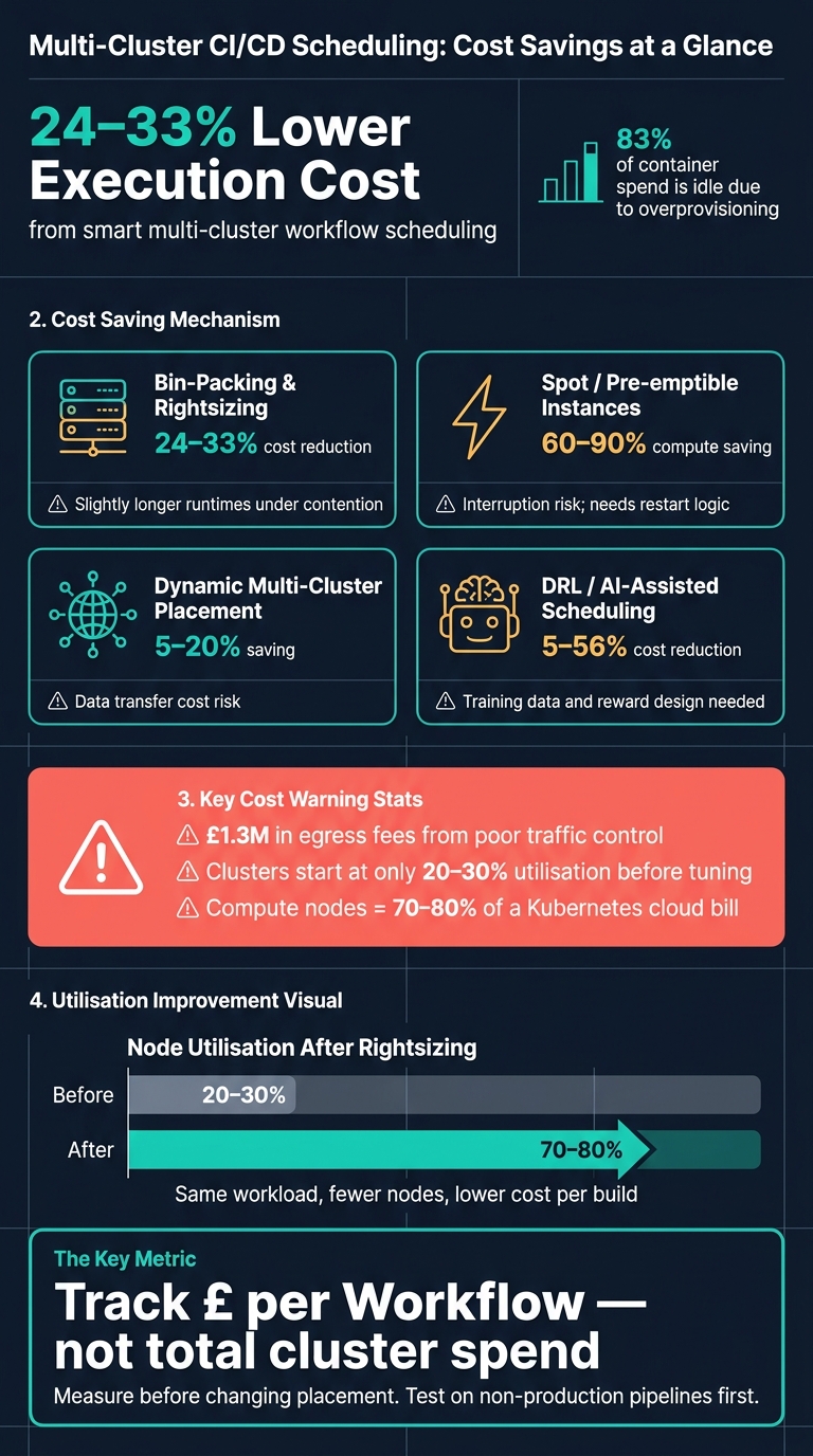 {Multi-Cluster CI/CD Scheduling: Cost Savings by Mechanism}
:::
{Multi-Cluster CI/CD Scheduling: Cost Savings by Mechanism}
:::
Kubernetes Multi-Cluster Consolidation Guide | Merge Clusters, Optimize Management & Reduce Costs
Quick comparison
| Area | What cuts cost | What adds cost | What I’d watch |
|---|---|---|---|
| Compute | Rightsizing, bin-packing, spot usage | Overstated requests, idle nodes | Node use, retry rates |
| Network | Data-local placement, registry mirroring | Cross-region or cross-cloud transfers | Egress per run |
| Cluster layout | Shared or hybrid pools | Full separation with spare capacity in each cluster | Idle baseline spend |
| Governance | Cost labels, policy checks, per-pipeline reporting | No controls, no audit trail | £ per workflow |
In short, I’d treat multi-cluster scheduling as a cost trade-off, not an automatic saving. The win comes from placing each job where the total cost is lowest, then proving it with per-run data.
2. What research shows about cost and performance trade-offs
2.1 Cost savings reported in scheduling research
Research points in the same direction: smarter scheduling can cut cloud spend, but the size of the win depends on how you schedule and what level of performance trade-off you're willing to accept.
The biggest savings usually come from three places: better use of existing capacity, cheaper interruptible compute, and placement that takes data locality into account.
Bin-packing and utilisation improvements tend to give the steadiest results. When workflows are packed onto fewer, better-used VMs, idle capacity drops and costs fall. The catch is fairly simple: denser packing can increase contention, which may slow tasks down.[2][3][1]
Spot and pre-emptible instances bring the sharpest price cuts. Compute spend can fall by 60–90% against on-demand pricing, but that only works for workloads that can survive interruption.[5][7] In research, schedulers deal with this by sending stateless jobs and easy-to-restart tasks to cheaper nodes, while keeping deadline-sensitive stages on steadier on-demand capacity.
Dynamic placement across multiple clusters or clouds tends to deliver smaller, but still useful, savings of 5–20%. The upside is that deadline performance can improve when placement decisions match data locality and billing model to the job.[1][6][8]
AI-assisted scheduling, especially deep reinforcement learning (DRL), can push costs down further. One DRL-based scheduler cut total costs by 5–56% against heuristic and competing DRL baselines, depending on how much SLA flexibility was available.[9] Another multi-objective RL scheduler achieved US$178 for 100 tasks, compared with US$195–US$210 for baseline models, while missed-deadline rates came in at 8.9% versus 10.2–17.3% for the baselines.[8] That said, AI schedulers are not magic. They need training data, and the reward setup has to be handled with care so the model does not lean too hard on cheap but unreliable nodes.
Here’s the short version:
| Mechanism | Typical Cost Saving | Primary Trade-off |
|---|---|---|
| Bin-packing and utilisation | 24–33% | Slightly longer runtimes under contention |
| Spot / pre-emptible instances | 60–90% on compute | Interruption risk; needs restart logic |
| Dynamic multi-cluster placement | 5–20% | Scheduling complexity; data transfer cost risk |
| DRL / AI-assisted scheduling | 5–56% | Training data needed; reward design risk |
2.2 How the research was conducted
Most of these studies rely on simulation-based experiments rather than live production pipelines. Researchers model VM pricing, task arrival patterns, and failure rates, then compare scheduling policies in controlled tests. That makes it easier to spot clear patterns - for example, denser packing lowers cost but can slightly increase makespan - though it doesn't reflect the constant churn of live CI/CD workloads all that well.
The optimisation methods also differ quite a bit.
Mixed-integer programming (MIP) produces strong theoretical results for smaller, tightly defined workloads, but it doesn't scale well to large, shifting fleets.[2][3][4][6] Metaheuristics such as genetic algorithms and ant colony optimisation, including the ProLiS and L-ACO algorithms, give up some optimality in exchange for scale. Studies show they can deliver lower execution costs and better deadline hit rates than older list schedulers across cloud workflow setups.[10] Reinforcement learning methods have also been tested on real edge and cloud platforms.[8]
For UK teams, the practical takeaway is straightforward. Treat MIP and simulation results as directional rather than plug-and-play. Heuristics and RL tend to transfer best when your workload looks like batch-heavy build and test pipelines. A sensible route is to try cost-aware heuristics inside your current scheduler first, test them against your own pipeline data, and then roll them out in stages.
These findings point to three main cost drivers: compute, data transfer and pipeline design.
3. The main cost drivers in multi-cluster CI/CD
The same workflow can cost very different amounts depending on where it runs, when it runs, and how clusters are set up. Compute, storage, and data transfer all shift with placement, timing, and topology. Then pipeline design decides how much avoidable work gets created in the first place.
3.1 Compute and utilisation: bin-packing, rightsizing, and pricing model mix
The biggest savings usually come from how jobs are packed and where they land. Compute nodes often make up 70–80% of a Kubernetes cloud bill[13][5], so anything that changes node utilisation has a huge effect on spend.
Here’s the catch: Kubernetes schedules pods based on requested resources, not actual usage. So if CI jobs ask for 4 vCPUs but usually use only one, the scheduler may place them on larger nodes and leave spare capacity sitting idle. You still pay for that idle space.
Most clusters sit at just 20–30% utilisation before any optimisation[11][5][12]. A focused rightsizing pass can change that fast. In plain terms, this means moving resource requests away from theoretical peak demand and closer to the 90th or 95th percentile of observed usage. Done well, that can push node utilisation up to 70–80%[11][15], which makes it possible to run the same workload on fewer nodes and cut cost per build.
Rightsizing often reduces compute spend without adding release risk, as long as limits are set properly.
Pricing model mix can push those savings further. Interruptible jobs belong on spot capacity, while release-critical stages should stay on stable nodes. That split keeps cheaper capacity doing the work that can tolerate disruption, without putting key delivery steps at risk.
There’s also a scheduler angle here. Kubernetes’ default scheduler tends to favour availability over dense packing[12][7][14][15]. If you switch to a MostAllocated scoring strategy, the scheduler packs more pods onto each node. That can change the bill in a very direct way.
Once compute is under control, the next leak tends to be cross-cluster data movement.
3.2 Data transfer, artefacts, and environment topology
Compute gets most of the attention, but network and storage costs are often where multi-cluster setups catch teams off guard. In multi-cluster CI/CD, placement decides whether a job stays near its registry, cache, and artefact store, or crosses a paid boundary.
Cloud providers usually don’t charge for data ingress, but they do charge for egress to the public internet on a per-GiB basis[16]. In practice, that matters every time a build agent pulls a large container image from a registry in another region, or when artefacts move from a test cluster to staging across availability zones or regions.
Co-locating your container registry and artefact store with your busiest CI cluster can cut egress costs and speed up image pulls. Registry mirroring helps too. If you keep a local copy of commonly used images close to the cluster doing the builds, bandwidth costs fall and pulls finish sooner. That can trim pipeline duration as well.
Environment topology shapes how these costs show up at scale. The table below compares the two common models:
| Model | Baseline Monthly Cost | Isolation | Elasticity | Scheduling Complexity |
|---|---|---|---|---|
| Separate clusters (dev, test, staging, prod) | Higher | Strong - clear boundary between environments | Lower - fragmented pools cannot share capacity | High - multiple schedulers and capacity plans |
| Shared cluster (namespaces per environment) | Lower | Moderate - enforced via RBAC, network policies, and taints | High - single resource pool responds to aggregate demand | Moderate - multi-tenancy controls to protect production-critical work |
| Hybrid (shared dev/test, separate prod) | Balanced | Strong for production, logical elsewhere | Good - dev/test pool scales freely | Moderate - two scheduling contexts to manage |
In practice, many UK organisations, especially in regulated sectors, end up with the hybrid model. Production stays on its own cluster for risk management and compliance, while development and testing share a cluster to keep baseline costs under control.
Even with smart placement, pipeline design still decides how much work the scheduler has to handle.
3.3 Pipeline design choices that waste or save money
Pipeline design and scheduling should be treated as one cost control, not two separate topics. The aim is simple: less demand. Fewer jobs, fewer artefacts, and less idle cluster time.
Conditional test execution helps by skipping full test suites when upstream changes don’t touch the relevant code paths. That cuts compute and storage use straight away. Test impact analysis goes a step further. It uses historical data to rank the tests most likely to fail for a given change, then defers or skips the lower-value ones.
Scheduled non-production shutdowns are another strong lever. For UK teams that work mostly to a 9-to-5 pattern, dev and test clusters often sit idle overnight and through weekends. Scaling them down, or switching them off during those periods, removes a steady source of waste.
These methods work best when they line up with scheduler behaviour. A light pipeline and a heavy pipeline should not be treated the same way. If you tag them clearly, the scheduler can place them on the right node types. You can also feed quiet periods into autoscalers so they scale down before idle time starts, not after.
Research shows that pairing workflow-level optimisation with cost-aware scheduling leads to bigger savings than using either one on its own, without measurable harm to release quality when backed by strong risk and test policies.
The table below maps common scheduling decisions to their cost and delivery effects:
| Scheduling Decision | Compute Effect | Storage/Network Effect | Deployment-Time Effect |
|---|---|---|---|
| Bin-packing (MostAllocated strategy) | Reduces node count by increasing utilisation per instance. | Minimal direct impact. | Can make scheduling less forgiving when capacity is tight. |
| Rightsizing resource requests | Lowers cost per build by reducing requested CPU/RAM. | Minimal direct impact. | Improves reliability by preventing OOMKills if limits are set correctly. |
| Spot/pre-emptible mix | Large reduction in hourly compute cost for eligible jobs. | No direct impact. | Requires retry logic and fail-fast design for interruptible stages. |
| Registry/artefact co-location | No direct impact. | Cuts egress and speeds image pulls. | Reduces latency for image-heavy pipeline stages. |
| Conditional test execution | Fewer jobs run; lower aggregate CPU and memory spend. | Fewer artefacts generated and stored. | Shorter pipelines; lower risk of blocking releases on irrelevant failures. |
| Non-production scheduled shutdown | Eliminates overnight and weekend idle node spend. | Minimal direct impact. | No effect on production. |
4. Cost-aware scheduling approaches UK teams can apply
The goal here is simple: run each job where it costs the least, then track the result in £ per pipeline run.
4.1 Dynamic job placement based on price, utilisation, and data locality
Take the cost drivers from earlier and turn them into placement rules. In practice, that means sending each job to the cluster or node pool where it is cheapest to run, based on live utilisation, price per vCPU-hour, and where the data already sits.
PIVOT placed tasks near their data source and cut subscription cost by over 55% and egress by up to 92% in comparative tests.[17]
For UK teams, region choice is not just about price. It also affects compliance. Workloads that handle personal data under UK GDPR must stay in approved UK or EU regions. A sensible way to handle this is to tag each pipeline by sensitivity and region, then enforce placement with cluster selectors and runner labels. If a job crosses regions, it should do so only when the drop in egress spend clearly beats the transfer cost. That means checking actual cloud pricing, not guessing that cheaper compute will always lead to a lower total bill.
There is a catch: these rules need care. Prices shift, cluster layouts change, and placement logic can drift over time.
When placement alone cannot cut enough spend, the next move is to run interruptible stages on spot-backed capacity.
4.2 Spot-backed and autoscaled execution for interruptible stages
Spot and pre-emptible node pools can cut costs by 30–70% on the right workloads, but only if those jobs can handle being interrupted.
Large batches of automated tests are often a good fit. That includes nightly regression suites, property-based tests, static analysis, and non-critical performance tests. These jobs tend to run in parallel, can be retried by the pipeline, and usually do not have strict completion deadlines. Production deploy stages are a bad fit. If a node disappears halfway through a deployment, you can end up with infrastructure in a half-applied state.
The safest pattern is a mixed-capacity autoscaling group. Keep a small pool of on-demand nodes for critical pipelines and as a fallback when spot capacity tightens. Then let spot nodes carry most of the interruptible work. Release workflows should get first access to on-demand capacity. Pipelines that run on spot pools also need to be idempotent, so they can restart cleanly from scratch, and they should use artefact caching so finished work does not need to be redone after a reclaim.
It also helps to watch interruption rates closely. If spot markets turn unstable, or if you are in a release window, move affected pipelines back to on-demand capacity.
The last piece is proof. To show that any of this works, teams need per-pipeline cost data and clear policy control.
4.3 Cost visibility, governance, and pilot rollout
Dynamic placement and spot-backed execution do not save money in a dependable way unless you measure the result. Without per-pipeline cost data, it is hard to tell whether a scheduling change lowered spend or just moved it somewhere else.
Tools such as OpenCost and Kubecost assign Kubernetes infrastructure spend - nodes, storage, and network - to individual pods and namespaces. Start with standard labels like pipeline=checkout, stage=test, and team=payments, then group spend by those labels in OpenCost or Kubecost. That gives you per-pipeline cost in £ per build or £ per test run, which is much easier to act on than raw node spend. Cloud dashboards can then fill in egress and storage costs that cluster tools may not show directly.
Governance matters just as much as visibility. Open Policy Agent (Gatekeeper) or Kyverno can enforce required labels at admission time, block unapproved regions for sensitive workloads, and limit how much spot capacity a given project may use. That helps stop scheduling rules from drifting as more pipelines get added.
For rollout, keep it small at first. Use a few non-critical pipelines, such as staging builds or nightly test suites, and record baseline metrics before changing anything:
- current £ per build
- average cycle time
- failure rate
Set success targets in advance. For example, aim for a 20% cut in per-test cost with no more than a 5% increase in retries. After a few weeks, review what happened, adjust the policy settings, and then extend the approach to more pipelines. Measurement, labelling rules, and policy-as-code are what make these savings stick.
The table below sums up how each approach compares for build, test, and deploy work.
| Approach | Typical Cost Reduction | Delivery Risk | Implementation Complexity | Build | Test | Deploy |
|---|---|---|---|---|---|---|
| Dynamic job placement | 10–30% | Medium - misconfigured placement can increase egress or breach compliance | High - requires labelling, cluster selectors, and policy upkeep | Strong | Strong | Limited - latency and compliance constraints apply |
| Spot-backed / autoscaled execution | 30–70% on eligible workloads | Medium–High - pre-emption risk requires solid retry and fallback design | Medium - mixed-instance groups and idempotent pipelines needed | Moderate for non-release builds | Strong | Poor for production; moderate for pre-production |
| Cost visibility & governance | 10–20% initially | Low - observability changes carry little delivery risk | Medium - labelling standards, tooling setup, and policy-as-code | Strong foundation for all stages | Strong foundation for all stages | Strong foundation for all stages |
5. Conclusion: Where multi-cluster scheduling cuts cost and where it adds overhead
The research points to a simple trade-off: the savings usually come from higher utilisation and smarter placement. One study found that 83% of container spend is idle due to overprovisioning[15]. In many cases, that’s where the biggest cost cuts sit.
The extra cost tends to come from duplicated fixed platform capacity and cross-cluster data transfer charges. So while multi-cluster scheduling can cut compute spend, it can also push up fixed platform and transfer spend by a similar amount.
That’s why the metric that matters isn’t cluster spend. It’s £ per workflow. Measure £ per workflow before changing placement, then test those changes on non-production pipelines for one release cycle.
Even then, the cheapest path isn’t always the right one. Lower-cost capacity in another region can help, but only if latency, interruption risk, and data residency stay within acceptable limits. Multi-cluster scheduling is a cost trade-off, not a guaranteed saving.
Hokstad Consulting can help UK teams build £-per-workflow cost models and put governance guardrails in place.
FAQs
How do I measure £ per workflow accurately?
Move past top-line invoices and tie costs to each workflow.
Use the same labels across namespaces and node pools, such as team, cost centre, and environment. That gives you a clean way to map spend back to the people and work behind it, instead of staring at one big cloud bill and guessing.
Then use Kubernetes cost tools like OpenCost or Kubecost to roll up pod- and namespace-level data. That makes it much easier to see which workflows are cheap, which ones are getting bloated, and where money is slipping away.
Bring these metrics into your CI/CD pipelines as well. Track compute use over time, flag costly re-runs, and watch for jobs that burn through resources without much to show for it.
It also helps to look beyond direct infrastructure spend. The bill from your cloud provider is only part of the picture. Indirect costs matter too, especially developer wait time when builds, tests, or deployments drag on.
Which CI/CD jobs are safe to run on spot nodes?
Spot instances are a good fit for fault-tolerant, non-critical CI/CD jobs that can cope with interruptions. That includes batch processing, CI runners, unit tests, and static analysis. Move this kind of work to spot nodes, and you can cut costs by 60–90% compared with on-demand pricing.
A simple way to think about it: keep your baseline capacity reserved, then use spot instances when workloads spike. More sensitive tasks, such as stateful services and control planes, should remain on on-demand instances.
When does multi-cluster scheduling increase costs?
Multi-cluster scheduling can get expensive fast when fixed cluster costs, day-to-day inefficiencies, and cross-cluster data movement start piling up.
Each Kubernetes cluster comes with control plane costs you can't avoid, even when workload levels are low. That means underused or duplicate clusters can quietly drain budget.
Costs climb further when scheduling doesn't account for network topology. In that case, workloads may trigger cross-zone egress fees that add spend without adding much value. On top of that, running multiple etcd instances or dealing with latency problems often creates extra operational overhead and pushes teams into over-provisioning.