
Cloud costs are a growing concern for businesses, with global public cloud expenditure expected to exceed $1 trillion by 2026. Yet, many organisations still rely on outdated forecasting methods, leading to budget variances of 25–40%. This impacts both overspending and underspending, creating inefficiencies and missed opportunities.
Here’s how to improve long-term cloud cost planning:
- Use Economic Models: Link cloud costs to business metrics like customer growth or transactions for better predictability.
- Understand Cost Drivers: Separate internal, external, strategic, and reduction drivers to identify where costs are rising or can be reduced.
- Adopt Unit Economics: Calculate costs per business output (e.g., per user or transaction) to track efficiency and eliminate waste.
- Forecast with Scenarios: Combine historical data with business events (e.g., product launches) for more reliable projections.
- Validate Regularly: Review assumptions monthly and track data accuracy to maintain forecast reliability.
Key Cost Drivers and Planning Variables
Core Cloud Cost Drivers
Cloud costs are influenced by a mix of internal, external, strategic, and reduction-related factors, all of which play a key role in shaping long-term financial models.
- Internal drivers: These include events like product launches, expanding into new regions, and scaling Kubernetes (automated adjustments for containerised workloads). These factors often lead to growth-driven increases in spending.
- External drivers: Factors such as vendor price adjustments and fluctuations in GBP/USD exchange rates can create unpredictable changes in unit costs.
- Strategic drivers: Actions like committing to Reserved Instances (long-term compute agreements) or adopting AWS Graviton processors can directly reduce unit compute costs.
- Reduction drivers: Activities such as decommissioning workloads or rightsizing resources lead to structural cost savings [5].
It’s essential to differentiate between rate optimisation (reducing unit costs through Savings Plans) and usage optimisation (cutting resource consumption). Confusing these can result in inaccurate forecasts [9].
These drivers form the basis of the unit economic framework, which we’ll delve into next.
Cloud Unit Economics
Tracking overall cloud expenditure isn’t enough. Unit economics links costs to the business outputs that drive them. The formula is straightforward: Total Cloud Costs ÷ Demand Driver Count. For example, a SaaS company might calculate costs per monthly active user, while an e-commerce platform could focus on costs per transaction [12].
Unit economics refers to the process of calculating the cost of a single unit of a business that can show the business value of the cloud.- Microsoft Learn [10]
This approach helps differentiate between efficient spending and wasteful practices. Without this perspective, finance teams may only see a rising overall spend, which doesn’t provide the full picture [11][13].
To measure cost efficiency, you can use the Cloud Efficiency Rate (CER) formula:
CER = (Revenue − Cloud Costs) ÷ Revenue × 100.
A CER of 85% or higher indicates strong cost efficiency, while a rate below 65% suggests cloud expenses are taking up too much revenue and need immediate action [12].
Impact and Volatility of Variables
A solid forecasting model requires a clear understanding of how predictable and impactful each cost variable is. The table below categorises these variables to help prioritise planning efforts [5][2]:
| Variable Category | Financial Impact | Predictability | Planning Focus |
|---|---|---|---|
| Fixed Baseline (RIs, Savings Plans) | High | High (95%+) | Contract management & utilisation |
| Growth-Driven (User/traffic growth) | High | Moderate (75–85%) | Unit economics & scaling factors |
| Project-Driven (New launches, migrations) | Moderate/High | Low/Moderate (50–70%) | Align with engineering roadmaps |
| External Drivers (Currency, price changes) | Variable | Low | Management buffers & quarterly reviews |
| Anomalies (Spikes, incidents) | Variable | Very Low (20–40%) | Statistical buffers & anomaly detection |
Fixed baseline costs are the most predictable and can be managed confidently through contracts and utilisation tracking. Growth-driven costs, however, require careful attention to unit economics and scaling assumptions. For project-driven expenses, aligning closely with engineering roadmaps is crucial. Meanwhile, external and anomalous costs are best managed with buffers rather than relying on precise predictions.
Don’t forget to account for seasonal trends, such as a 20% traffic surge during peak retail periods, to adjust for predictable fluctuations [5].
Need help optimizing your cloud costs?
Get expert advice on how to reduce your cloud expenses without sacrificing performance.
Cloud unit economics: Making unpredictable cloud costs easier to forecast [#132)
Modelling Techniques for Long-Term Cloud Cost Projections
::: @figure 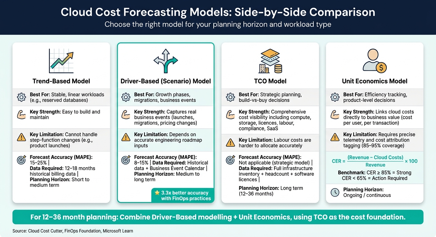 {Cloud Cost Forecasting Models Compared: Which One Is Right for You?}
:::
{Cloud Cost Forecasting Models Compared: Which One Is Right for You?}
:::
Once you've identified your cost drivers and variables, the next step is selecting the right model to forecast them. There's no universal solution - the choice depends on how steady your workloads are, the pace of your business growth, and how far into the future you're planning.
Baseline Trend Models
Trend-based models are a straightforward starting point. They use 12–18 months of historical billing data to project future costs by extending current growth patterns [3]. These models are ideal for workloads that are stable and predictable, such as reserved databases or infrastructure with consistent utilisation.
A common approach is to follow the Model Ladder
. Begin with simple moving averages to establish a baseline, then progress to exponential smoothing for workloads with seasonal variations. Machine learning models should only come into play when you're dealing with complex, multi-variable cost drivers [2]. Jumping into ML without solid baseline data can overcomplicate your analysis unnecessarily.
The primary drawback of trend models is their inability to predict step-function changes - major events like product launches, regional expansions, or architectural shifts can render trend-based projections inaccurate [3][9]. For situations where historical data can't account for abrupt changes, scenario-based models offer a more adaptive solution.
Scenario-Based Models
Scenario-based (or driver-based) models incorporate business context alongside historical data [3]. Instead of merely extending a trend line, these models simulate specific events, such as a new product launch in Q3, a migration off legacy systems, or the expiration of a pricing commitment that alters your cost structure.
Organisations with strong FinOps practices achieve 3.3x better forecast accuracy by combining trend and driver-based methods.- Cloud Cost Cutter [3]
A helpful tool for this approach is a Business Event Calendar, which tracks anticipated events like peak retail periods or planned migrations. Without this, models may misinterpret expected spikes as anomalies, leading to inaccurate variance reports [2][7]. Driver-based models generally achieve a Mean Absolute Percentage Error (MAPE) of 8–15%, compared to 15–25% for pure trend-based models [2]. This improved accuracy is crucial when planning Savings Plans or Reserved Instances.
Beyond simply forecasting costs, integrating these models with business outcomes enables more advanced analyses like TCO (Total Cost of Ownership) and unit economics.
Unit Economics and TCO Models
Building on the unit economics framework, this method ties cloud expenditure directly to business outcomes, rather than just predicting raw costs.
A TCO model captures the complete cost of running cloud infrastructure - not just compute and storage, but also software licences, engineering labour, compliance expenses, and third-party SaaS subscriptions [1][4]. The unit economics model refines TCO by linking these costs to key business metrics, creating a direct connection between spending and performance [1][7].
These two models complement each other rather than serving as substitutes. The table below highlights their differences:
| Model | Best For | Key Strength | Key Limitation |
|---|---|---|---|
| Trend-Based | Stable, linear workloads | Easy to build and maintain | Can't handle step-function changes [3] |
| Driver-Based (Scenario) | Growth phases, migrations | Captures real business events | Depends on accurate roadmap inputs [3][9] |
| TCO Model | Strategic planning, build-vs-buy decisions | Comprehensive cost visibility, including labour | Labour costs are harder to allocate [1][4] |
| Unit Economics Model | Efficiency tracking, product-level decisions | Links costs to business value | Requires precise telemetry and attribution [1][7] |
For long-term planning (12–36 months), combining driver-based modelling with unit economics works best. Use TCO as the foundation for costs and business metrics as a lens for efficiency. This approach helps finance and engineering teams align on whether cloud investments are delivering proportional value.
Inputs, Assumptions, and Data Validation
A model's reliability depends heavily on the quality of its data. Before diving into any forecasting exercise, it’s essential to carefully consider what data you’re gathering, its sources, and how reliable your assumptions are.
Data Required for Projections
The backbone of any cloud cost forecast is historical billing and usage data. For medium-term forecasts, aim for at least 12–18 months of data, while long-term planning requires 18–36 months. Using daily data is crucial as it captures patterns like weekday vs. weekend usage and month-end spikes, which can be missed with monthly summaries [5].
You’ll also need commitment data, such as Reserved Instances (RIs), Savings Plans (SPs), utilisation rates, and expiration dates. Without this, there’s a risk of underestimating future costs [7][9].
Additionally, include business signals like product launches, geographic expansions, or engineering migrations. These can be sourced from internal roadmaps and change logs, as they often drive sudden and significant cost changes [6][3].
For accurate cost attribution and efficiency tracking, aim for 85–95% tagging coverage across dimensions like environment, team, application, and project. Poor tagging can lead to inaccurate projections and missed opportunities to optimise costs [2].
Testing and Validating Assumptions
Once data collection is sorted, the next step is to rigorously test and validate the assumptions that underpin your forecast.
To ensure precision, regularly update growth and pricing assumptions. A proven method for validation is sequential backtesting: train your model on an earlier data set, forecast the next period, and then move the training window forward. This approach helps reveal how well your model adapts to real-world changes, avoiding the mistake of inadvertently using future data in training [7][2].
The difference isn't complex algorithms; it's having a repeatable process, clean data, and the right validation framework.- Vishnu Siddarth, Opsolute [2]
Different assumptions require different review schedules. For example:
- Growth rates tied to user acquisition or traffic should be reviewed monthly.
- Efficiency targets, like rightsizing results or storage tiering, need quarterly reviews.
- Pricing forecasts also need quarterly updates, especially since AWS has adjusted its pricing more than 100 times since its inception [5].
- Commitment coverage, such as SP or RI utilisation, requires weekly or monthly reviews due to the financial stakes involved.
| Assumption Group | Validation Frequency | Key Data Points |
|---|---|---|
| Growth Rates | Monthly | User acquisition, traffic volume, data growth |
| Efficiency Targets | Quarterly | Rightsizing outcomes, unit cost trends |
| Pricing Forecasts | Quarterly | Provider rate changes, new instance types |
| Commitment Coverage | Weekly/Monthly | SP/RI utilisation, expiration dates, savings rates |
If variance exceeds 10%, it’s a signal to immediately investigate the root cause. This could stem from new workloads, pricing adjustments, or misconfigured services [6][5].
Ensuring Data Quality
Improving data quality has a more immediate effect on forecast accuracy than the complexity of the model itself. Research shows that organisations without structured cost management waste 32–40% of their cloud budgets [3], and poor data hygiene can lead to forecast errors of 20–40% [5].
To improve accuracy:
- Normalise multi-cloud billing data into a unified format (e.g., date, service category, resource ID, cost, and tags). This ensures that data from AWS Cost and Usage Reports (CUR), Azure Cost Management exports, and GCP BigQuery billing can be compared consistently [5].
- Adjust for calendar effects by normalising monthly data to a per-day basis. For instance, comparing February (28 days) to March (31 days) without adjustment will distort trends [2].
- Add an anomaly buffer of 10–15% of the baseline to account for unexpected incidents or experimental workloads [5].
- Set budget alerts at 50%, 80%, and 100% of forecasted spend to catch overruns early, rather than discovering them at the end of the month [3].
Building and Refining the Forecast
Forecast Construction Workflow
With reliable data and solid assumptions in hand, the next step is to build, monitor, and manage a forecast that supports long-term planning. Start by breaking down total cloud spend into two categories: predictable costs (like Reserved Instances, Savings Plans, and fixed subscriptions) and volatile costs (such as bursty compute usage and data egress) [14]. From there, focus on forecasting costs per active user, per API call, or per transaction, aligning projections with business growth rather than simply relying on past expenditures [15]. To prepare for demand fluctuations, create three forecast scenarios: Conservative, Expected, and Aggressive [14][15]. When making commitments, aim for 90% of the lower limit of the forecast's 95% confidence interval - this helps minimise the risk of overcommitting [2].
Cloud bills do not move in a vacuum. They are shaped by demand growth, regional energy costs, hardware pricing cycles, and broader inflation trends.- ComputerTech.cloud [14]
Use statistical methods to develop and refine your baseline forecast [2]. Following this approach can significantly reduce budget variance, bringing it down from 25–40% to less than 10% [2]. Once the model is in place, set up systems to validate and adjust the forecast regularly.
Ongoing Validation and Refinement
After launching the forecast, continuous validation becomes essential. By day 10, identify any variances to allow for a two-to-three-week window to make necessary adjustments [2]. If variances exceed your target threshold, investigate why the model underperformed.
Optimisation efforts must be included in forecasts to maintain trust in the model. Otherwise, variance will show up as unexplained.- FinOps Foundation [8]
Advanced FinOps teams operating at the Run
level aim for a quarterly forecast variance of less than 10–12% [15][8]. The table below outlines key validation steps to incorporate into your process:
| Validation Checkpoint | Frequency | Key Metric / Action |
|---|---|---|
| Variance Review | Weekly | Compare actual vs. forecast (WAPE/MAPE) [8] |
| Assumption Tuning | Monthly | Update drivers – launches, decommissions, growth rates [8] |
| Anomaly Audit | Real-time | Investigate spikes; distinguish structural shifts from one-offs [8] |
| Unit Economics Review | Monthly | Track cost per business unit (e.g., cost per transaction) [16] |
| Model Refresh | Daily | Ingest latest billing data to keep the baseline current [8] |
Be mindful of bias traps like Survivorship Bias (focusing only on current architecture while ignoring retired services) and Target Leakage (using data unavailable at prediction time). These can undermine forecast accuracy without raising obvious red flags [7].
Governance and Reporting
Once the forecast is built and fine-tuned, integrate it into your operational governance to ensure timely decision-making. Static forecasts that are rarely reviewed won't be effective. Instead, make forecasts actionable by embedding them into your cloud governance processes. Use forecasted-to-breach alerts, which trigger when current spending trends indicate a future budget overrun, to shift from reactive to proactive management [8][6].
Run Budgets and Anomaly Detection together. One shows the trend. The other flags the surprise.- Erik Peterson, AWS Optics Team Lead [8]
Tailor reporting to your audience. Engineers need detailed, service-level variance data, while finance teams and leadership require scenario comparisons and summaries of commitment coverage. Where feasible, link forecast alerts to specific application or environment owners in your CMDB to ensure clear accountability [8]. Establish a governance routine with weekly variance reviews and monthly updates to assumptions, keeping forecasts reliable and actionable across the organisation.
How Hokstad Consulting Supports Long-Term Cloud Cost Planning
When it comes to building a dependable long-term cloud cost strategy, having expert guidance is essential to turn detailed models into actionable plans.
Cloud Cost Engineering Expertise
Creating a solid long-term cloud cost model isn’t easy, especially with constantly changing infrastructures. Hokstad Consulting excels in cloud cost engineering, helping businesses cut cloud expenses by 30–50%. They achieve this through in-depth cost audits, financial modelling, and precise optimisation efforts. Instead of relying on generic solutions, they dig into billing data to identify spending inconsistencies, establishing a clear cost baseline - a crucial step for any meaningful long-term forecast.
Their expertise spans the entire cost engineering process, from spotting underused resources and adjusting commitments to crafting unit economics frameworks. These frameworks link cloud costs to business outcomes, ensuring finance and engineering teams can communicate effectively. This approach eliminates the disconnect that often exists between financial forecasts and technical budgets.
Tailored Long-Term Planning Support
Every business has unique long-term cloud needs. Hokstad Consulting offers services like DevOps transformation, strategic cloud migration, and managed hosting, all designed to support multi-year strategies rather than quick fixes. This aligns with the financial models previously discussed, ensuring financial and technical teams are on the same page.
Their zero-downtime migration strategy accurately models transition costs, making multi-year projections more reliable. For companies shifting from legacy systems to cloud-native solutions, this structured migration process ensures architectural changes are deliberate and well-organised, avoiding last-minute, reactive decisions.
Custom Automation for Forecasting
Manual forecasting can quickly become unmanageable at scale. Hokstad Consulting addresses this by creating automated tools that process live billing data and detect forecast discrepancies early. Using advanced statistical methods, they handle non-linear cost trends and account for factors like seasonal and holiday fluctuations [17]. This is especially useful for UK retail and other seasonal industries, where demand can vary significantly throughout the year.
They also employ Adaptive Laddering to manage commitments automatically, reducing the risk of underused or expired Reserved Instances - a frequent source of unexpected costs in long-term cloud environments [9]. These automated solutions provide consistently reliable and accurate cost projections, ensuring businesses stay ahead of potential budget surprises.
Conclusion and Key Takeaways
Long-term cloud cost planning replaces guesswork with precision by using structured economic models. Without these models, forecasts can deviate by 20–40%. However, employing layered techniques like scenario modelling, unit economics, and regular validation can cut that variance to under 10% [2][5].
The main takeaway here is simple: your cloud forecast should be a living, adaptable tool, not a static spreadsheet updated once a year. Regular practices, such as weekly variance reviews, monthly model updates, and maintaining a robust four-layer forecast structure (Fixed Baseline, Growth-Driven, Project-Driven, and Anomaly Buffer), ensure your projections stay grounded as your infrastructure changes [5]. These steps help keep your forecasts in sync with your business needs.
The goal isn't perfection, it's actionable insights that drive smarter, data-backed financial decisions.- Opsolute [2]
Accurate inputs are just as important as the forecasting model itself. Key factors like macroeconomic signals (e.g., the Consumer Price Index), disciplined tagging with 85–95% coverage, and an up-to-date business event calendar all play a critical role in making your forecasts reliable [2][14]. These aren't just optional improvements - they're the difference between a forecast that withstands Q3 traffic spikes and one that collapses under unexpected growth.
If you're ready to shift from reactive cost management to proactive financial planning, Hokstad Consulting can help. Their expertise in cloud cost engineering - from building unit economics frameworks to deploying automated forecasting tools - empowers finance and engineering teams with a unified, dependable view of long-term cloud spending.
FAQs
Which cloud cost model should we use first?
To kick off cloud cost modelling, a seasonal time-series model is a great choice. It's straightforward to implement, easy for finance teams to grasp, and provides clear insights.
Start by zeroing in on the key cost drivers, such as:
- API requests
- Data transfer (measured in GB per month)
- Instance-hours
- Storage usage
Use metrics from a typical week to establish a baseline. From there, adjust your model to account for variations during peak and off-peak periods. This approach helps in creating a more accurate and adaptable cost framework.
What’s the best demand driver for unit economics?
When identifying the best demand driver for unit economics, focus on a business-centred metric that reflects the value your company provides and ties directly to revenue. Avoid technical metrics like compute hours, as they don't clearly connect to outcomes. Instead, opt for an outcome-focused unit, such as a paying customer, a completed transaction, or a billable API call.
This approach makes cost data more actionable and provides better insight into how scaling impacts infrastructure expenses. Ultimately, the ideal unit will depend on your specific business model and what drives value for your company.
How do we set the right anomaly buffer?
To create a practical anomaly buffer, consider including a modest management reserve in your budget. This reserve, calculated as a percentage, can help absorb minor fluctuations without needing constant revisions. Implement programmatic budgets with step-based alert thresholds to monitor actual spending and predict potential overruns effectively. According to Hokstad Consulting, pairing these reserves with clean historical data - free from anomalies, deleted resources, and one-off expenses - can significantly enhance forecasting precision and keep your budget on track.