
How you access data in the cloud matters more than how much you store. This article breaks down five common data access patterns - row-oriented, column-oriented, key-value, time-series, and graph - and explains their cost and performance trade-offs. Here's the key takeaway: the right pattern depends on your workload, not a one-size-fits-all solution.
Key Points:
- Row-oriented: Best for transactional tasks (e.g., MySQL, PostgreSQL). Cost-efficient for single-row operations but expensive for analytics due to excess data reads.
- Column-oriented: Ideal for analytics (e.g., ClickHouse, Snowflake). Scans less data and achieves better compression but struggles with single-row updates.
- Key-value: Suited for high-speed object retrieval (e.g., Amazon S3). Simple and scalable but incurs costs from frequent small-file operations.
- Time-series: Handles sequential, timestamped data well (e.g., DynamoDB, Timestream). Efficient with tiered storage but requires careful partitioning.
- Graph: Great for relationship-heavy queries (e.g., social networks). Costs rise with traversal depth and high write volumes.
Quick Comparison:
| Pattern | Cost | Performance | Scalability | Complexity |
|---|---|---|---|---|
| Row-oriented | High for analytics | Fast reads, slower writes | Limited for large datasets | Simple for transactions |
| Column-oriented | Variable (depends on query) | High throughput for analytics | Scales well for large datasets | Moderate setup effort |
| Key-value | Moderate to high | Sub-millisecond response | Excellent for object retrieval | Simple, but key design matters |
| Time-series | Low with tiering | High for sequential reads | Excellent with partitioning | Moderate automation needed |
| Graph | High (depth-dependent) | Slower with complex queries | Moderate (I/O spikes possible) | High due to query tuning |
Pro Tip: Reduce costs by eliminating unnecessary reads, optimising file sizes (128–512 MB), and using tiered storage for older data. Each pattern has strengths and weaknesses - choose based on your specific needs and budget.
::: @figure 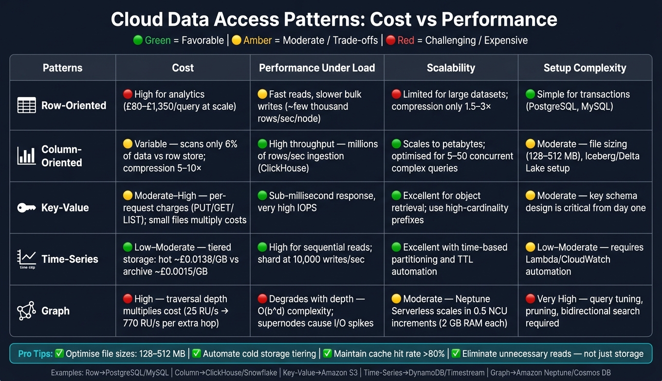 {Cloud Data Access Patterns: Cost vs Performance Comparison}
:::
{Cloud Data Access Patterns: Cost vs Performance Comparison}
:::
Are your cloud queries burning cash? Here is how to optimize.
1. Row-oriented access patterns
Row-oriented databases, like PostgreSQL and MySQL, arrange complete records together on disk. This design is great for fetching and updating entire rows quickly, but it can become inefficient when you only need data from a few columns in a large table.
Cost
For transactional tasks - things like point lookups, single-row inserts, or updates - row stores are very efficient. A single-row update involves just one B-tree traversal and one page read, keeping latency low.
But analytical queries are a different story. Row stores read all the data in a row, even if only a few columns are needed. For instance, querying 3 columns in a 50-column table might require reading around 400 MB of data in a row store, compared to just 24 MB in a column store. This difference adds up, especially with serverless query engines charging roughly £4 per TB scanned. For large datasets, like 100 billion rows, compute costs for analytical scans can range from £80 to £1,350 per query [2][6]. While row stores are cost-efficient for transactional tasks, they can become expensive for analytics due to unnecessary data reads.
Load handling
Row stores thrive in handling high-concurrency transactional workloads. For example, Google AlloyDB has demonstrated handling about 467,000 transactions per second on certain tasks, while PlanetScale's sharded MySQL clusters handle over 420,000 queries per second for transactional traffic [2]. However, bulk write throughput is a weakness. Most row stores hit their limits at a few thousand rows per second per node. This bottleneck stems from the need to maintain indexes and manage Write-Ahead Logs (WAL).
The OLTP write path optimises for one-row-at-a-time durability; the OLAP write path optimises for throughput.- Al Brown, ClickHouse [2]
Scalability
Row stores are excellent for transactional tasks, but as datasets grow into the billions of rows and analytical queries become more frequent, their performance starts to lag. Tasks that take seconds on column stores may stretch into minutes or even hours on row stores [3][6]. Compression is another factor - row stores typically achieve compression ratios of 1.5–3×, whereas column stores can reach 5–10×. This means storage costs for row stores increase faster as data grows [2].
Setup complexity
One of the strengths of row stores is their simplicity. Tools like PostgreSQL and MySQL are well-documented, widely supported, and relatively easy to configure for most needs [3]. The complexity arises when trying to use row stores for analytical purposes. Techniques like creating covering indexes to mimic column store behaviour can add significant maintenance challenges. For straightforward transactional tasks, row stores are a great starting point. However, as analytical demands grow, transitioning to a column store might become necessary [3].
2. Column-oriented access patterns
Column-oriented databases, unlike their row-based counterparts, are designed for selective and highly compressed data reads. This approach offers notable advantages in terms of cost and performance. Databases like ClickHouse and Snowflake, along with file formats such as Parquet and ORC, store data by columns rather than rows. This design drastically reduces the volume of data scanned during a query, leading to significant cost savings.
Cost
Imagine querying just 3 columns from a table with 50 columns. In a column-oriented system, you'd only scan about 6% of the data compared to a row-based database. Additionally, columnar formats often achieve compression ratios of 5× to 10×, with low-cardinality columns sometimes compressing up to 30× [2][8]. With serverless query pricing at roughly £4 per terabyte scanned, these savings can add up quickly, especially when dealing with large datasets.
However, using SELECT * in systems like BigQuery forces the engine to scan every column, negating these I/O savings and increasing costs [4]. When working with massive datasets, the efficiency of columnar systems becomes particularly evident, as discussed further in the load-handling section.
Load handling
When it comes to bulk ingestion, columnar engines are in a league of their own. For instance, ClickHouse can ingest millions of rows per second per node - far surpassing the single-digit thousands typically handled by row-oriented systems [2]. This is made possible by vectorised execution, which processes data in batches using SIMD (Single Instruction, Multiple Data), achieving speeds of hundreds of millions of rows per second per core [8].
However, these systems aren't as efficient for single-row updates or deletes, as these operations require rewriting entire compressed blocks. To address this, many systems buffer small writes in a row-oriented delta store
before compacting them into the column store in larger batches [2][8]. These traits make columnar databases highly scalable, but with specific design considerations.
Scalability
Columnar storage is well-suited for scaling into terabyte and even petabyte ranges. This is because the amount of data read is tied to the number of columns accessed, rather than the total width of the table [2]. Sorting data by frequently queried fields, such as date or customer_id, further optimises performance by narrowing the min/max statistics stored in file footers, allowing engines to skip irrelevant data blocks entirely [7][9].
That said, columnar systems are typically optimised for a smaller number of complex queries running simultaneously - usually between 5 and 50 - rather than thousands of simple lookups [3].
Columnar databases are terrible for OLTP workloads, and row databases are terrible for OLAP workloads at scale. This is not a minor preference; it is a fundamental architectural mismatch.- CloudRPS Blog [3]
Setup complexity
Getting the most out of columnar storage requires careful setup. Managing file sizes is critical, with uncompressed files ideally falling between 128 MB and 512 MB. Files smaller than 10 MB can create excessive metadata overhead, hurting performance [5]. Partitioning data, such as by date, can also help query optimisers skip irrelevant partitions entirely.
To simplify operations at scale, formats like Apache Iceberg and Delta Lake have become popular. These frameworks build on raw Parquet or ORC files, adding features like ACID transactions and manifest-based pruning [5]. While they streamline management, they do come with their own learning curve, requiring time and effort to master.
3. Key-value access patterns
Key-value (KV) stores, like Amazon S3, focus on simplicity and scalability, making them ideal for handling high-volume, discrete object retrieval. Unlike row and column stores, KV mechanisms are designed for fast storage and retrieval of immutable objects. They perform particularly well for use cases like high-volume event ingestion - think clickstream data, IoT telemetry, or ad-impression logs. They also handle multi-tenant workloads effectively, ensuring operational isolation.
Cost
The cost of using a KV store is heavily influenced by access patterns rather than just the volume of data stored. Every operation - whether it’s a PUT, GET, or LIST request - comes with a charge. If your workload involves frequent access to many small files, costs can quickly add up. This is because managing small files introduces additional metadata indexing overhead, which acts as a cost multiplier.
To manage these costs, it’s crucial to batch writes into files sized between 128–512 MB. Files smaller than 32 MB can significantly increase metadata overhead, further driving up costs[1][5].
Load handling
Amazon S3 automatically scales request capacity, but it doesn’t happen instantaneously. During sudden traffic spikes, you might encounter HTTP 503 Slow Down
responses as the system works to allocate new internal partitions[10]. To avoid these bottlenecks, key design plays a critical role. Sequential or time-ordered prefixes like logs/2026/05/16/... can overload a single partition, creating performance issues. Instead, use high-cardinality prefixes - such as tenant IDs or hex hashes - to distribute the load evenly across partitions[10][11].
Scalability
KV stores shine when it comes to point lookups and object retrieval, but they aren’t the best choice for scan-heavy analytics. For analytical workloads, columnar formats like Parquet are far more efficient[5]. However, KV patterns excel in multi-tenant architectures. By starting keys with high-cardinality dimensions, such as tenant IDs, you can achieve horizontal scalability while maintaining strong operational isolation[10].
Setup complexity
In KV systems, the key itself serves as the sole schema. There are no secondary indexes, joins, or query planners - just a string that guides routing within a distributed system[10]. While this simplicity is a strength, it also means that designing the key structure correctly from the beginning is crucial. Decisions around lifecycle rules, access policies, and partitioning strategies all hinge on this initial design. Attempting to fix a poorly designed key schema at scale can be both complex and expensive.
These insights into key-value patterns pave the way for understanding the unique challenges of managing time-series data, particularly in terms of cost and performance.
4. Time-series access patterns
Time-series data tends to follow a consistent pattern: it’s written quickly, queried frequently when new, and accessed rarely as it ages [12]. This predictable behaviour makes it ideal for tiered storage solutions, but it also comes with its own set of cost and performance challenges.
Cost
One of the biggest cost factors in time-series systems is the overhead from data ingestion. For instance, Amazon Timestream charges a minimum of 1 KB per ingestion request, no matter how small the actual payload is [16]. Thomas Landgraf from Industrial-Grade Architecture highlights this issue:
AWS Timestream accounts for a minimum of 1 KB per ingestion, regardless of the actual payload size.[16]
To reduce ingestion costs, you can buffer data using tools like Amazon SQS and batch writes before sending them. For query costs, always include a time filter in the WHERE clause, as serverless models typically charge around £4 per TB of data scanned [5]. Storage tiering also offers savings: moving older data from hot storage (around £0.0138 per GB) to archive storage (about £0.0015 per GB) can significantly cut costs.
By combining these strategies, you can better manage the expenses tied to high ingestion rates and frequent queries.
Load Handling
High ingestion rates, such as 10,000 writes per second, can create bottlenecks if all writes are directed to a single partition key. Sharding - adding a random suffix to distribute writes across multiple partitions - helps alleviate this issue [14]. For DynamoDB, on-demand writes cost around £1.25 per million write request units, while provisioned capacity costs approximately £0.65 per WCU-hour [14]. Additionally, enabling native Time-to-Live (TTL) features ensures expired records are automatically purged, keeping storage usage efficient without manual clean-up.
These load-handling techniques are essential for maintaining smooth operations as data volumes grow.
Scalability
Amazon Timestream’s serverless architecture is well-suited for workloads with unpredictable spikes. For NoSQL systems like DynamoDB, you can create separate tables for different time periods (e.g., daily or monthly) to balance the need for high write capacity on recent data with lower demand for older records [12]. While on-demand capacity offers simplicity, it can be about 30% more expensive than provisioned capacity with auto-scaling during steady traffic [14]. Another way to optimise performance is by downsampling data - pre-computing one-minute averages, for example - to minimise the need for re-scanning large datasets in long-range queries [5].
Setup Complexity
Managing time-series data efficiently often demands more automation compared to other data models. Tools like AWS Lambda and CloudWatch Events can automate tasks such as table management, capacity adjustments, and TTL configurations [12]. However, high-cardinality datasets - those with millions of unique tag combinations - can strain memory and slow down compaction processes [15]. To address this, keep cardinality low and use specialised functions like max_by(value, time) to retrieve the latest values, reducing both memory usage and query complexity [13].
These approaches highlight the balance required between cost, performance, and operational complexity when working with time-series data.
5. Graph access patterns
Graph access patterns shed light on the balance between cost and performance in cloud data management. Graph databases are particularly effective for handling data rich in relationships - think social networks, fraud detection systems, or recommendation engines. However, this strength often comes with added expenses and complexity.
Cost
The cost of graph access patterns is heavily influenced by traversal depth. Each extra hop in a traversal can dramatically increase operation counts. For example, in Azure Cosmos DB, a single traversal using the Gremlin API costs about 25 RU/s, but doubling the traversal depth can push this to around 770 RU/s. By contrast, re-modelling graph data into a NoSQL structure for simple one-hop queries can reduce this cost significantly, with double traversals dropping to just 11–15 RU/s [17].
As Subhasish Ghosh, a Cloud Solution Architect at Microsoft, explains:
This approach is not recommended if you are mostly doing a 2x- and 3x- or more level of traversals with complex edge-relationships and/or data size of database is > 5 TBs.[17]
The choice of approach depends on the specific query profile and workload, as these cost factors directly influence performance and load management.
Load Handling
Graph databases can face challenges with high write volumes, particularly in serverless solutions like Amazon Neptune Serverless. During bulk data ingestion, replication lag may occur, causing reader instances to fall behind the primary writer. AWS suggests either temporarily disabling reader instances during heavy loads or setting the maximum capacity to 128 NCUs to ensure sufficient throughput. For spiky workloads, serverless instances can offer considerable savings, potentially cutting costs by approximately £3,076.20 per month compared to large provisioned instances [18].
These load-handling strategies are critical for maintaining performance and ensuring graph systems scale effectively over time.
Scalability
Amazon Neptune Serverless provides fine-grained scalability, allowing adjustments in 0.5 NCU increments, with each unit offering 2 GB of memory. This flexibility makes it well-suited for unpredictable traffic patterns. However, as Kevin Phillips, Neptune Specialist Solutions Architect at AWS, points out:
For workloads where traffic is consistent, using a serverless instance will be cost-inefficient compared to using a provisioned instance of the same capacity.[18]
For analytical tasks - such as large-scale trend analysis - using a separate in-memory graph analytics engine can prevent resource contention with transactional databases [19]. The scalability decisions you make will directly influence the complexity of maintaining optimal performance in graph systems.
Setup Complexity
Graph queries can become computationally intensive, especially when dealing with multi-hop traversals. These grow at a rate of O(b^d), where b is the average fan-out and d is the number of hops. Highly connected supernodes
can exacerbate the issue, causing significant I/O spikes. Techniques like degree-aware pruning and bidirectional search (when both the source and target are known) can effectively halve traversal depth and reduce the number of operations. Additionally, proactive query tuning - such as early filtering and transaction batching - can help manage ongoing maintenance demands [20].
As Lee Razo, Sr. Cloud Partner Architect at Neo4j, aptly summarises:
Multi-hop queries stop being 'search' and become 'work generators': a single extra hop often multiplies traversals by an order of magnitude.[20]
Pros and Cons
Each access pattern - row, column, key–value, time-series, and graph - comes with its own mix of cost and performance challenges. The best choice depends on your workload, budget, and how much operational complexity you’re willing to handle. Interestingly, most cloud expenses aren’t driven by storage volume alone. Instead, request fees and metadata overhead often end up being the real cost drivers [1].
Here’s a quick comparison table that highlights the key trade-offs for each access pattern:
| Access Pattern | Cost | Performance Under Load | Scalability | Setup Complexity |
|---|---|---|---|---|
| Row-oriented | High (provisioned IOPS & capacity) | Slower writes, fast reads | Limited by latency | High (network/consistency tuning) |
| Column-oriented | Variable (request fees dominate) | High throughput for large scans | High (via partitioning & compaction) | Moderate (schema evolution, file compaction) |
| Key-value | Moderate to high due to reliance on volatile memory | Sub-millisecond response, very high IOPS | High (asynchronous replication) | Moderate (cache invalidation, TTL management) |
| Time-series | Low–moderate (cold tiering helps) | High for sequential reads | High (time-based partitioning) | Low–moderate (retention policies) |
| Graph | High (costs multiply with traversal depth) | Performance declines significantly as traversal depth increases | Moderate (supernodes can cause I/O spikes) | Very high (query tuning, pruning strategies) |
Key-value and in-memory patterns are great for lightning-fast responses, with sub-millisecond latency and high IOPS. However, they can be expensive because they depend heavily on RAM. To keep costs under control, aim for a cache hit rate of at least 80%. Anything lower can lead to unnecessary expenses [21]. On the other hand, graph patterns excel in handling relationship-heavy data but become costly and slower as traversal depth increases.
Another important factor is the balance between compute and storage. For example, deleting intermediate datasets to save on storage might seem smart, but it often backfires. Recomputing that data can increase read operations and drive up compute costs, sometimes outweighing the storage savings [1]. In fact, poor visibility and overprovisioning are responsible for up to 30% of cloud spending being classified as waste [22].
You don't optimize cloud storage by deleting data - you optimize it by eliminating unnecessary reads.- The Data Forge [1]
For businesses in the UK, understanding these trade-offs is essential. Expert advice, such as that offered by Hokstad Consulting (https://hokstadconsulting.com), can help you design a cloud architecture that balances performance needs with cost-efficiency. These considerations lay the groundwork for the final conclusions.
Conclusion
Looking at row-oriented, column-oriented, key–value, time-series, and graph access patterns, it’s clear that no single approach fits every workload. Row-oriented patterns work well for transactional systems, while column-oriented ones are ideal for large-scale analytical queries. Key-value stores provide lightning-fast speeds for high-throughput caching, time-series patterns manage sequential, time-stamped data efficiently and affordably, and graph patterns excel at handling complex, relationship-heavy queries, though they can become more expensive as query depth increases.
Choosing the right data access pattern is about more than just performance - it’s also about managing costs effectively. A poor choice can lead to unnecessary expenses, such as oversized instances or inefficient partitioning. To keep costs in check, aim for analytic file sizes between 128–512 MB, automate lifecycle transitions to colder storage tiers, and maintain a cache hit rate above 80%.
Balancing cost and performance is crucial, especially in modern architectures that often combine multiple patterns. This added complexity can escalate quickly, making expert guidance invaluable. Hokstad Consulting offers specialised cloud cost engineering services, claiming to reduce cloud expenses by 30–50% through precise audits and optimisations. With their No Savings, No Fee model, teams can explore cost-saving opportunities without upfront financial risk.
Ultimately, the goal isn’t about choosing the cheapest or fastest pattern but finding the right fit for your data, your users, and your budget.
FAQs
How do I choose the right data access pattern for my workload?
Choosing the right data access pattern involves weighing up cost, performance, and the specific demands of your workload. Synchronous replication is a good fit for critical systems, as it guarantees strong consistency. However, it comes with higher costs and slower write speeds. On the other hand, asynchronous replication prioritises faster writes and lower costs, though it compromises on immediate consistency, making it better suited for workloads where this trade-off is acceptable. Additionally, using caching and aligning resources with regional requirements can help fine-tune performance and manage costs effectively in certain environments.
What changes cut cloud data costs fastest without hurting performance?
The fastest way to cut cloud data costs while maintaining performance is by using automated data tiering and strategic caching. Automated tiering shifts data to more budget-friendly storage tiers depending on how often it’s accessed. Meanwhile, caching places frequently used data closer to users. These techniques work together to reduce storage and network expenses, enhance response times, and keep data easily accessible.
When should I use a mix of patterns instead of just one?
Using a variety of data access patterns is a smart way to strike the right balance between cost and performance for different workloads or components within an application. For example, you can schedule non-critical tasks using cost-effective methods while prioritising high-performance strategies for critical services. Similarly, pairing caching for frequently accessed data with traditional storage solutions helps lower costs without sacrificing speed. This customised approach is especially effective in managing the demands of complex cloud environments, ensuring both consistent performance and efficient resource use.